Open Crime data are very powerful for predictive crime analyses. Most Police units make use of historical data and GIS to analyze crime patterns and trends. The conclusion drawn from these analyses are used to better place officers more efficiently on the field, for example.

We think it is very interesting to show how historical crime data can be used to analyse crime patterns in space and time, and to present the results to the local authorities. We found the very intersting Open Data Portal of the city of Tulsa, OK, for our analyses. The city provides crime data in Shapefile for the period 2010 – 2014.

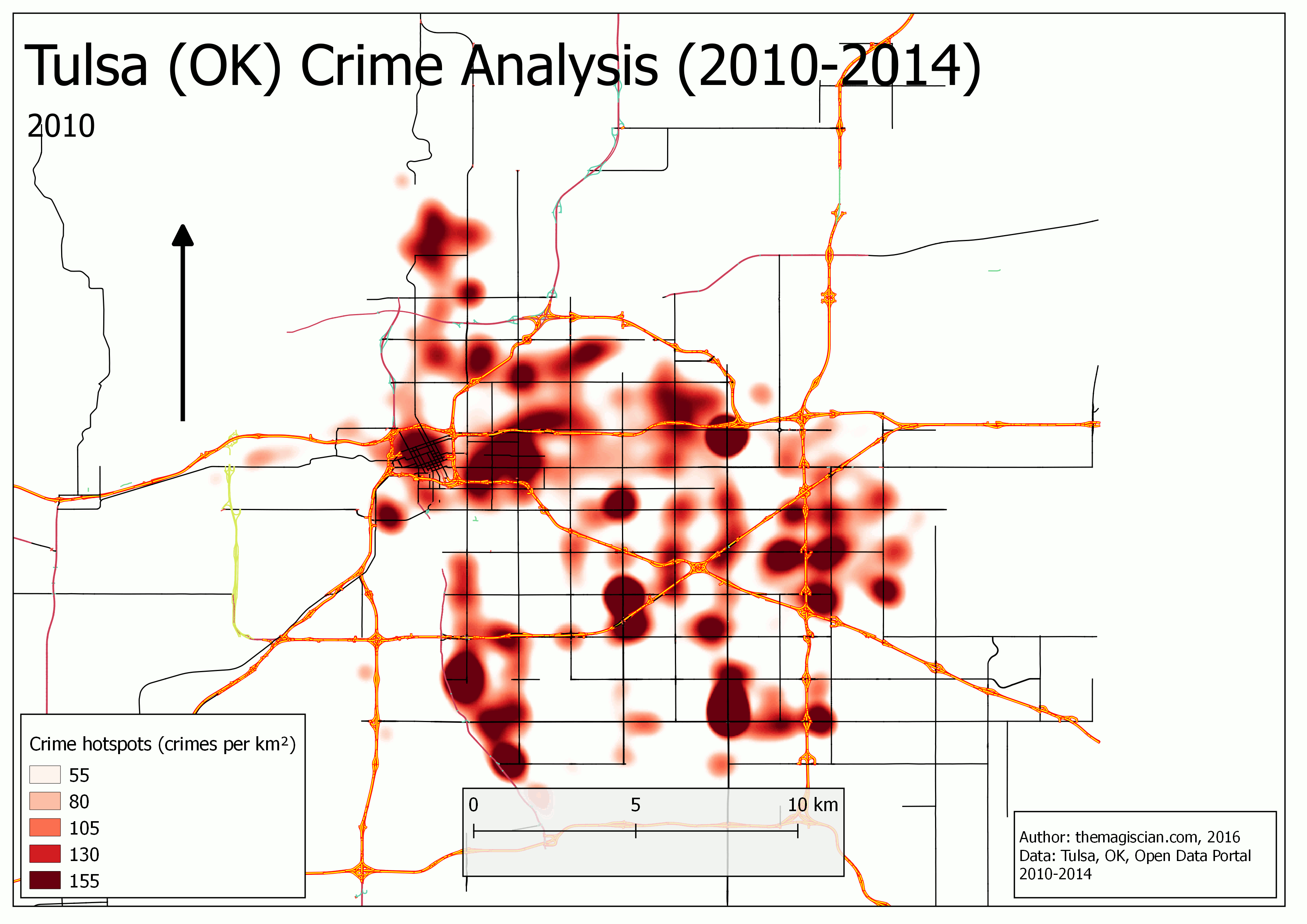
See how the crimes spread accross the city for the study period. Notice already some crime hotspots!

Let’s play around with these data and do deeper analysis!

Data structure

There is a Shapefile for every year of the study period. The model of all the Shapefile is as followed.

The fields we are interesting in are the following:
ucc_crime1
start_date
start_day
start_time
end_date
end_day
end_time

The location matters also of course. What we want to do through these analyses are to place the crime data on a map and to perform more fine-grained analyses for depicting patterns and trends.

We’ve decided to add the road network of the city in order to situated things on the maps. The road data is coming from OpenStreetMap.

Data loading and preparation

As for always, we’re working with a PostGIS database.

Create first the database.

CREATE DATABASE tulsa_crime WITH OWNER themagiscian;

If needed, enable the PostGIS extension.

CREATE EXTENSION postgis;

Data loading

The following shp2pgsql command uploads the Shapefiles into the database.

shp2pgsql -s4269 -d -ggeom -S -I "<PATH>\Crimes_2014.shp" public.crimes | psql -Uthemagiscian -h<ip-address> -dtulsa_crime
shp2pgsql -s4269 -a -ggeom -S -I "<PATH>\Crimes_2013.shp" public.crimes | psql -Uthemagiscian -h<ip-address> -dtulsa_crime 
shp2pgsql -s4269 -a -ggeom -S -I "<PATH>\Crimes_2012.shp" public.crimes | psql -Uthemagiscian -h<ip-address> -dtulsa_crime 
shp2pgsql -s4269 -a -ggeom -S -I "<PATH>\Crimes_2011.shp" public.crimes | psql -Uthemagiscian -h<ip-address> -dtulsa_crime 
shp2pgsql -s4269 -a -ggeom -S -I "<PATH>\Crimes_2010.shp" public.crimes | psql -Uthemagiscian -h<ip-address> -dtulsa_crime 
shp2pgsql -s4326 -d -ggeom -S -I "<PATH>\osm_roads.shp" public.roads | psql -Uthemagiscian -h<ip-address> -dtulsa_crime

Data preparation

The fields that contain the date are not in a DATE format. We need to make sure it is because we’ll need to perform analyses based on time. Notice that the data for which there’s an “Unknown” for the end_date have been changed to a NULL value.

ALTER TABLE CRIMES ALTER COLUMN start_date TYPE DATE 
using to_date(start_date, 'MM/DD/YYYY');

ALTER TABLE CRIMES ALTER COLUMN start_time TYPE TIME 
using start_time::time;

ALTER TABLE CRIMES ALTER COLUMN end_date TYPE DATE 
using to_date(end_date, 'MM/DD/YYYY');

UPDATE crimes SET end_time = NULL WHERE end_time = 'Unknown';

ALTER TABLE CRIMES ALTER COLUMN end_time TYPE TIME 
using end_time::time;

For the road data from OSM, we do not need some of the attributes. We drop them.

-- Structure roads table
ALTER TABLE roads DROP waterway;
ALTER TABLE roads DROP aerialway;
ALTER TABLE roads DROP barrier;
ALTER TABLE roads DROP man_made;

Analyses

Let’s first see how much crimes were registered in the 2010-2014 period.

SELECT count(*) FROM CRIMES; count
 --------
 139139

For a city of about 400 000 citizen, it makes an average of 87 crimes per 1000 person per year. Which is pretty high.

Per crime type

How does the total number of crimes decline in the different crime types?

SELECT ucc_crime1 CRIME_TYPE, count(*) TOTAL_CRIMES FROM CRIMES GROUP BY ucc_crime1 ORDER BY total_crimes desc;

We then create a distinct view for each of these crime type to make further queries easier.

CREATE VIEW CRIMES_TYPE_LARCENY AS SELECT * FROM CRIMES WHERE ucc_crime1 = 'LARCENY';
CREATE VIEW CRIMES_TYPE_BURGLARY AS SELECT * FROM CRIMES WHERE ucc_crime1 = 'BURGLARY';
CREATE VIEW CRIMES_TYPE_MALICIOUS_MISCHIEF AS SELECT * FROM CRIMES WHERE ucc_crime1 = 'MALICIOUS MISCHIEF';
CREATE VIEW CRIMES_TYPE_AUTO_THEFT AS SELECT * FROM CRIMES WHERE ucc_crime1 = 'AUTO THEFT';
CREATE VIEW CRIMES_TYPE_AGGRAVATED_ASSAULT AS SELECT * FROM CRIMES WHERE ucc_crime1 = 'AGGRAVATED ASSAULT';
CREATE VIEW CRIMES_TYPE_ROBBERY AS SELECT * FROM CRIMES WHERE ucc_crime1 = 'ROBBERY';
CREATE VIEW CRIMES_TYPE_RAPE AS SELECT * FROM CRIMES WHERE ucc_crime1 = 'RAPE';
CREATE VIEW CRIMES_TYPE_HOMICIDE AS SELECT * FROM CRIMES WHERE ucc_crime1 = 'HOMICIDE';

Where do these crimes mostly occur?

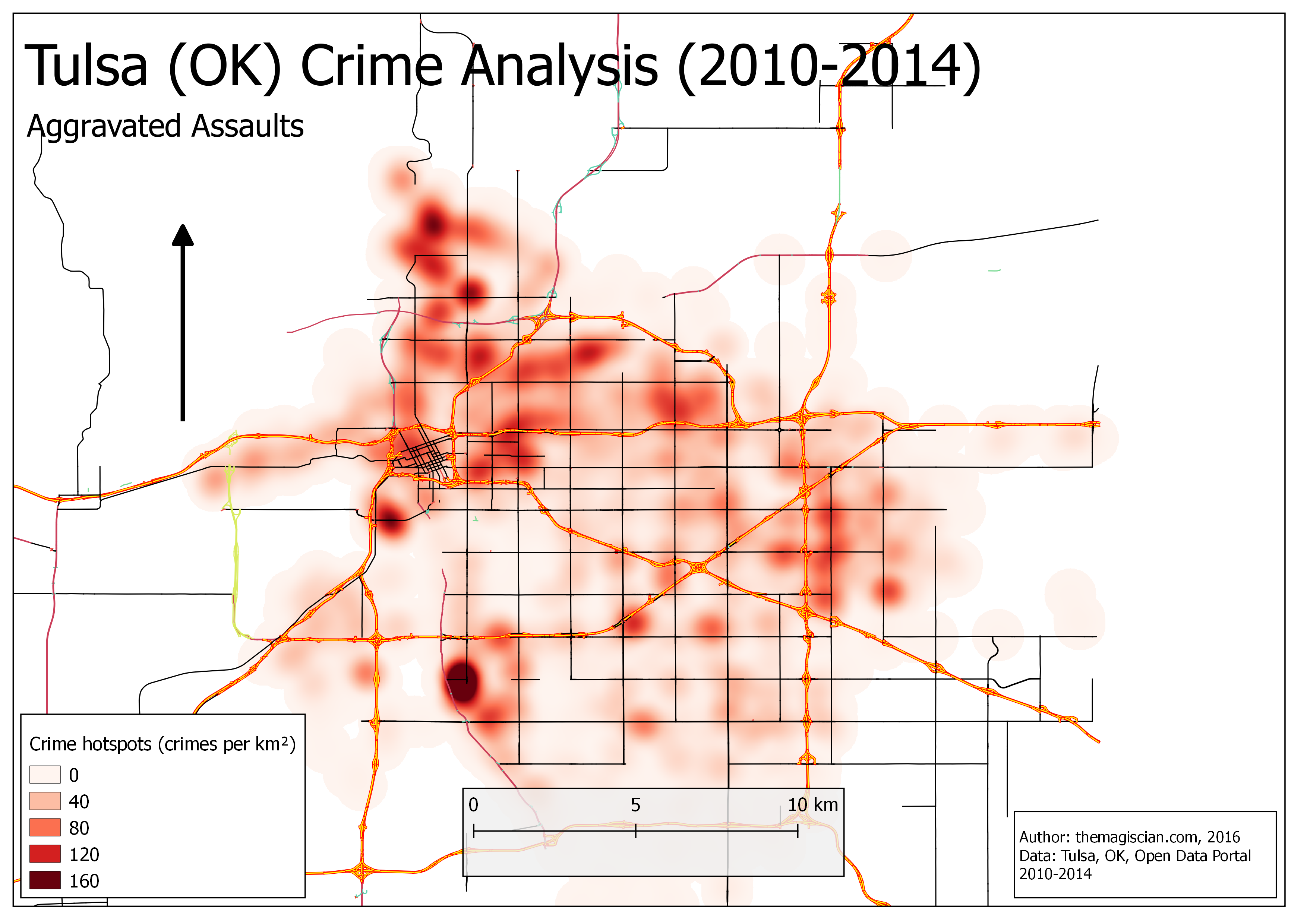
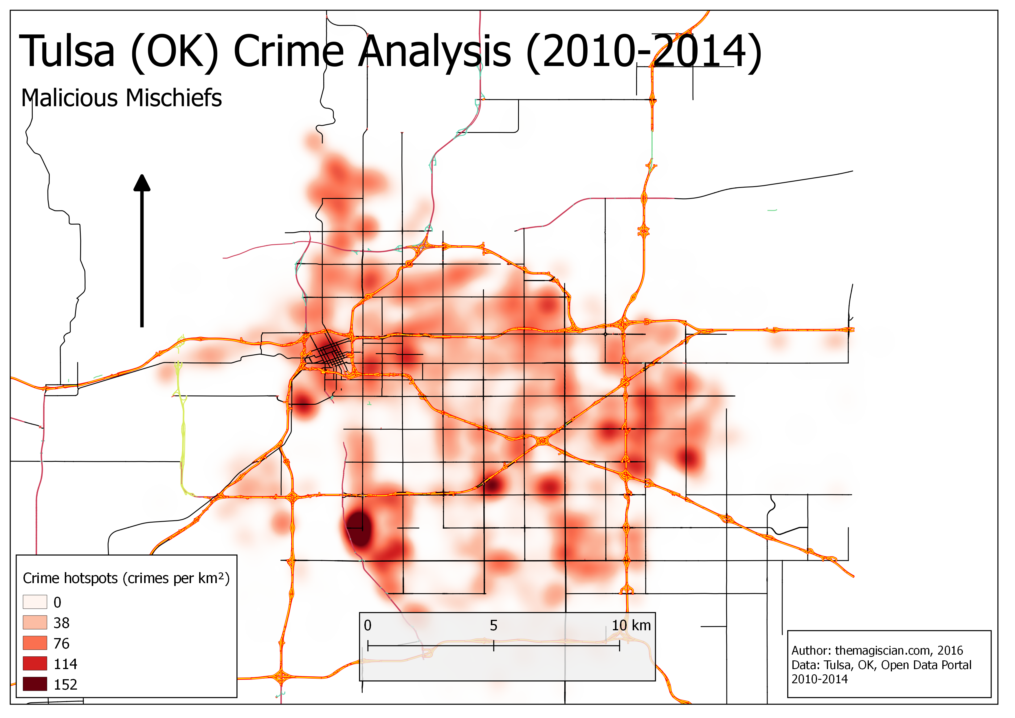
Using QGIS, and plotting the crimes of the map, we were able to create the following maps to see where all these different crimes occur. Pay attention to the color scales for each maps which are different.

Notice that these maps have been done using the Heatmap functionnality in QGIS. See here the tutorial that was followed.

We won’t comment each of the cases but we will describe our point of view about the most frequent hospots at the end.

Aggravated Assaults

Auto thefts

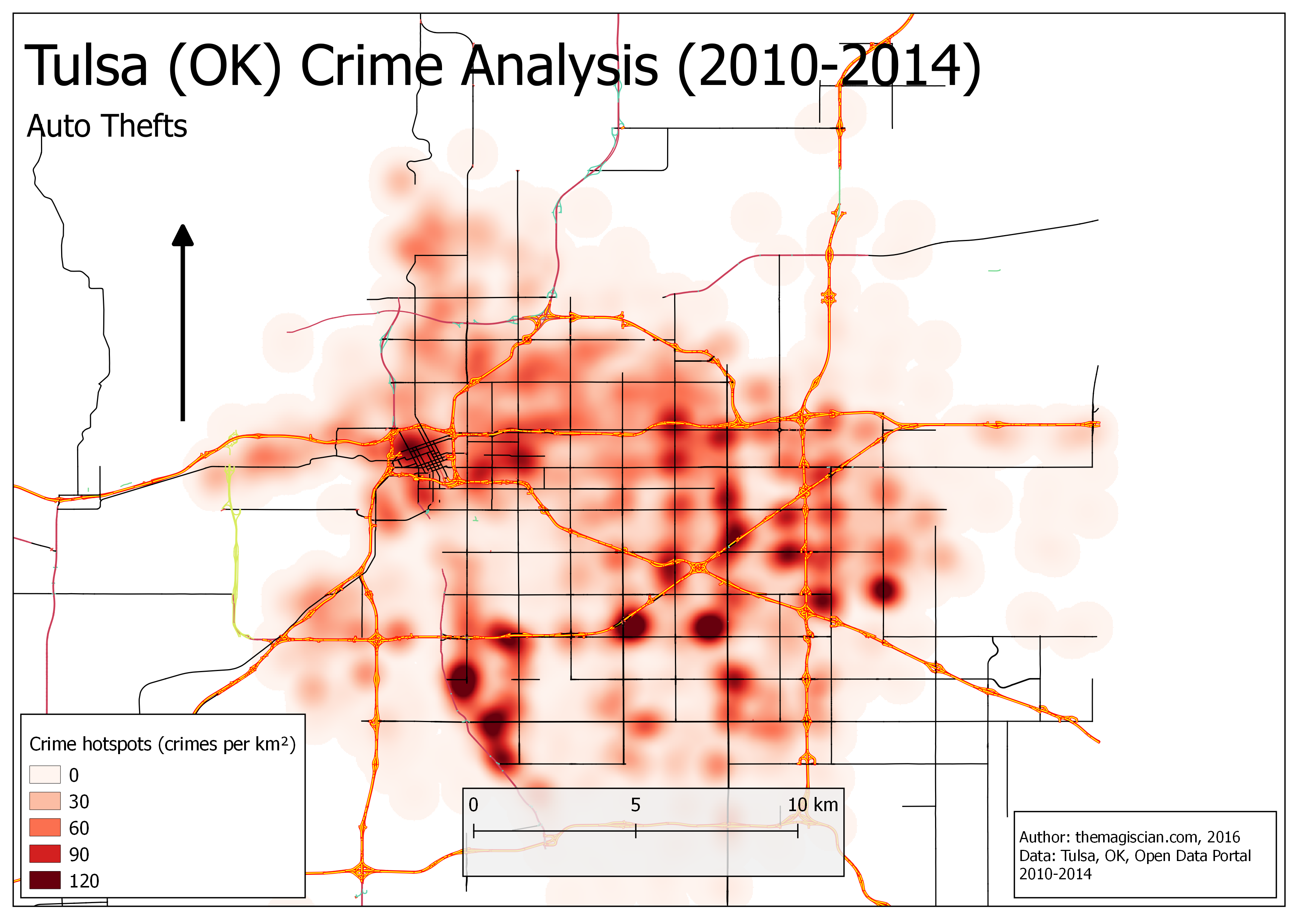
Auto thefts crimes tend to be more homogeneously spread accross the city.

Burglaries

Homicides

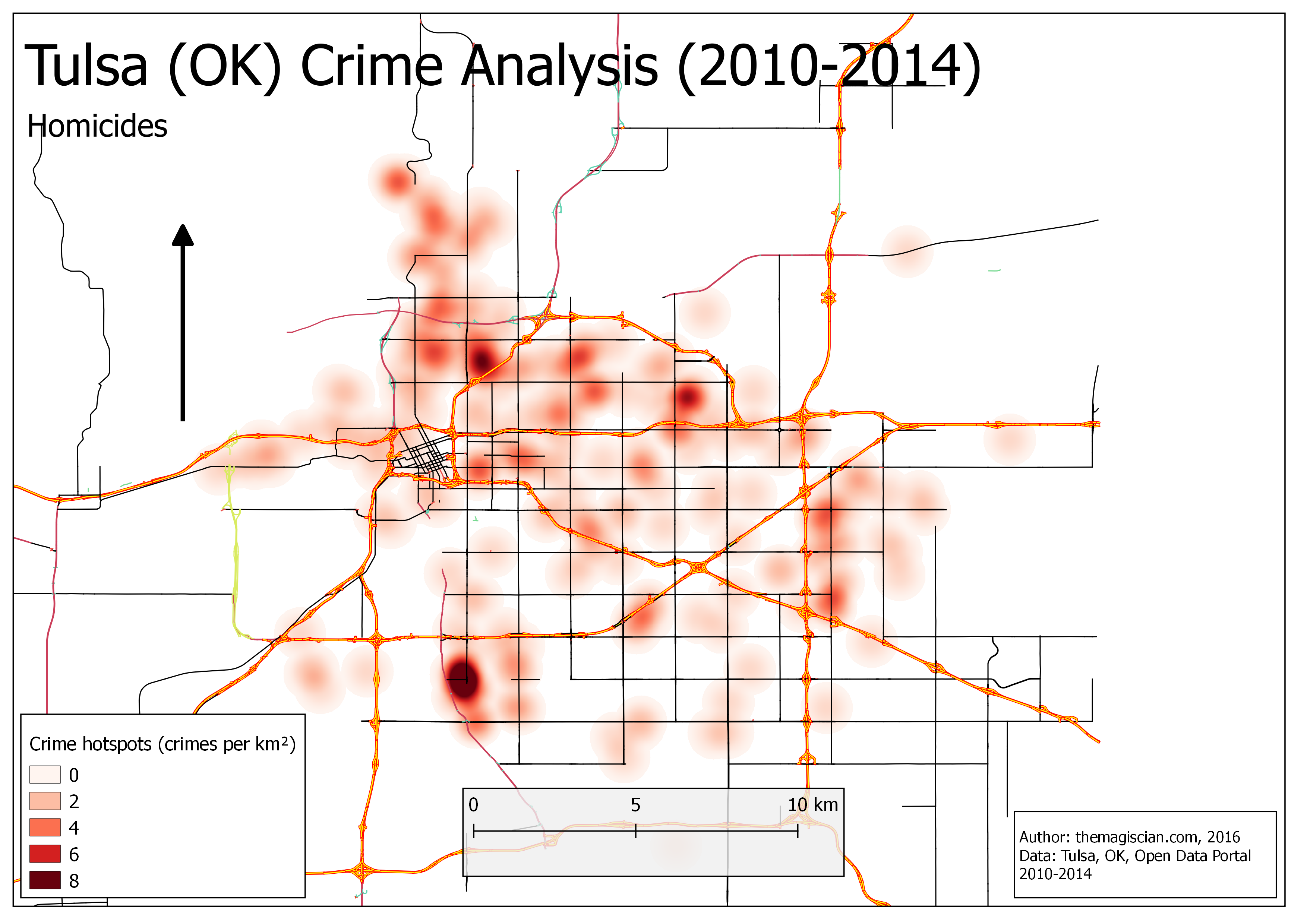
A very obvious hotspot appears in the South of the city of Tulsa. Let’s stop here to see what happens. Using QGIS, we were able to identify a spot where 4 people were killed.

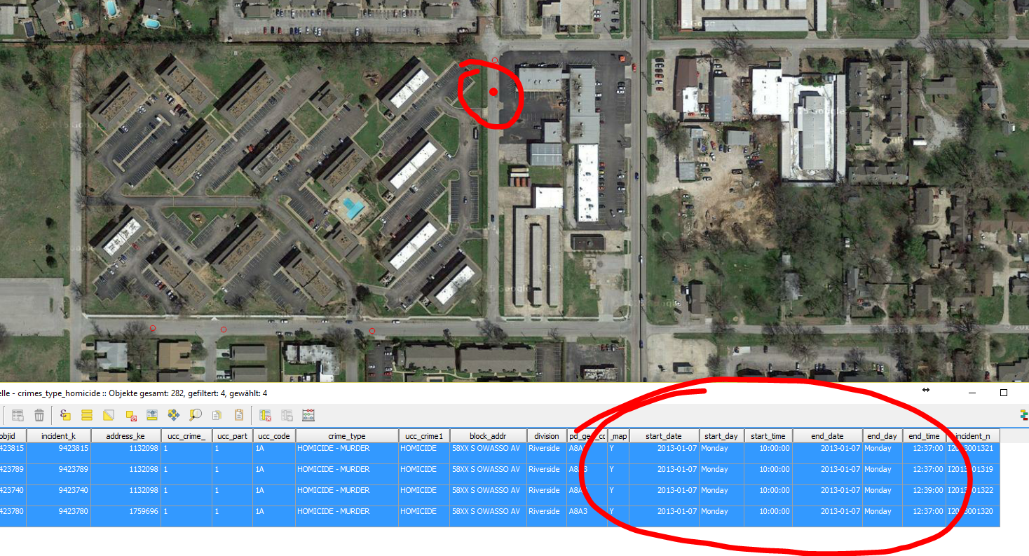
Searching on the internet, we found evidence for what was happening.

Larcenies

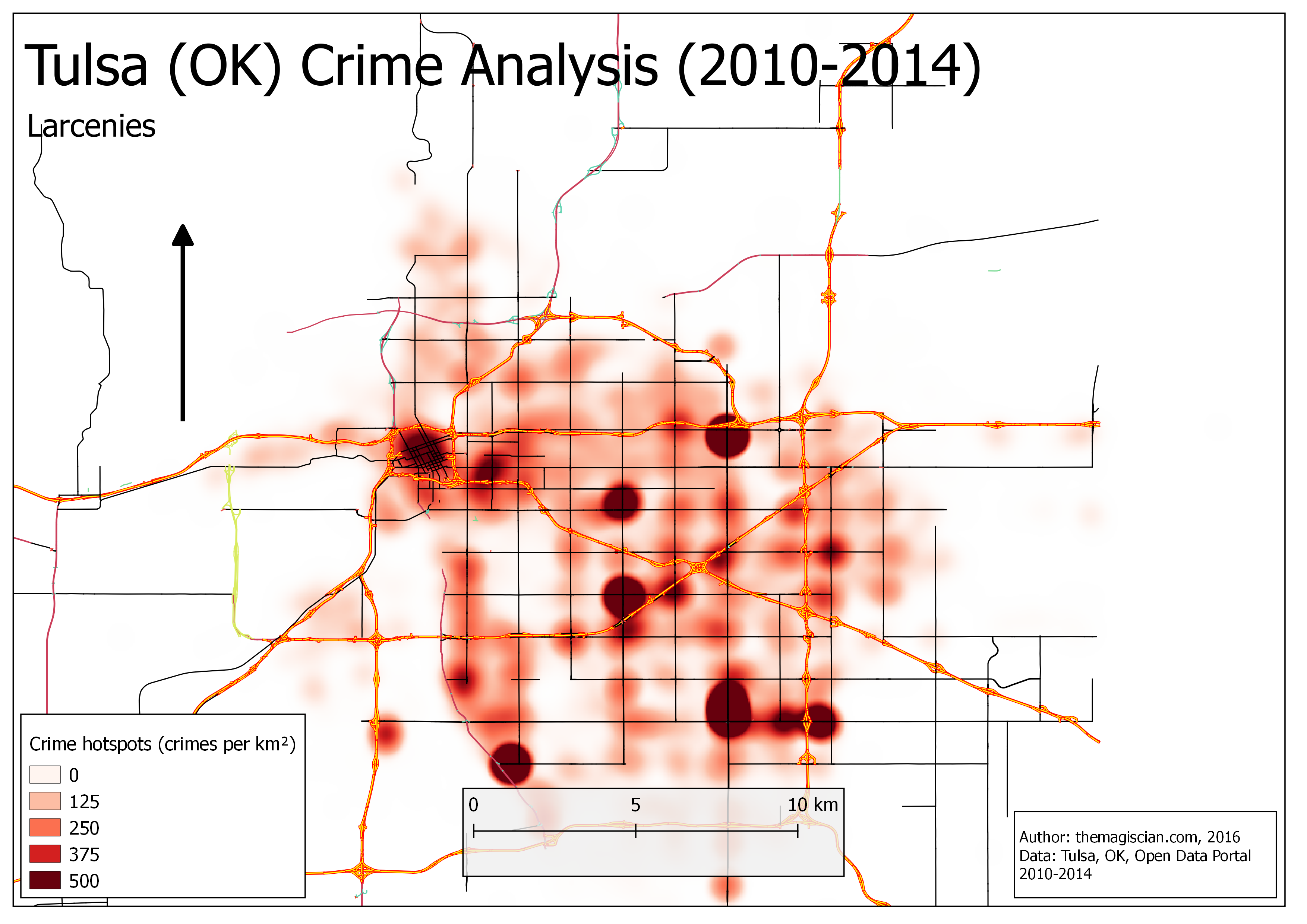
Some hotspots are very clear. In the South-East of the city. We see there 3 big spots (from West-to East): The Woodland Hills Mall, Sam’s Club and then an area with a Target and an Eastside Market among others. In the North-East, we have a big Walmart.

In general, all these areas very crowded places and are shopping malls. Except for the spot in the South-West, which is a University Campus. Notice also the high rate of larcenies in Downtown.

Malicious Mischiefs

Rapes

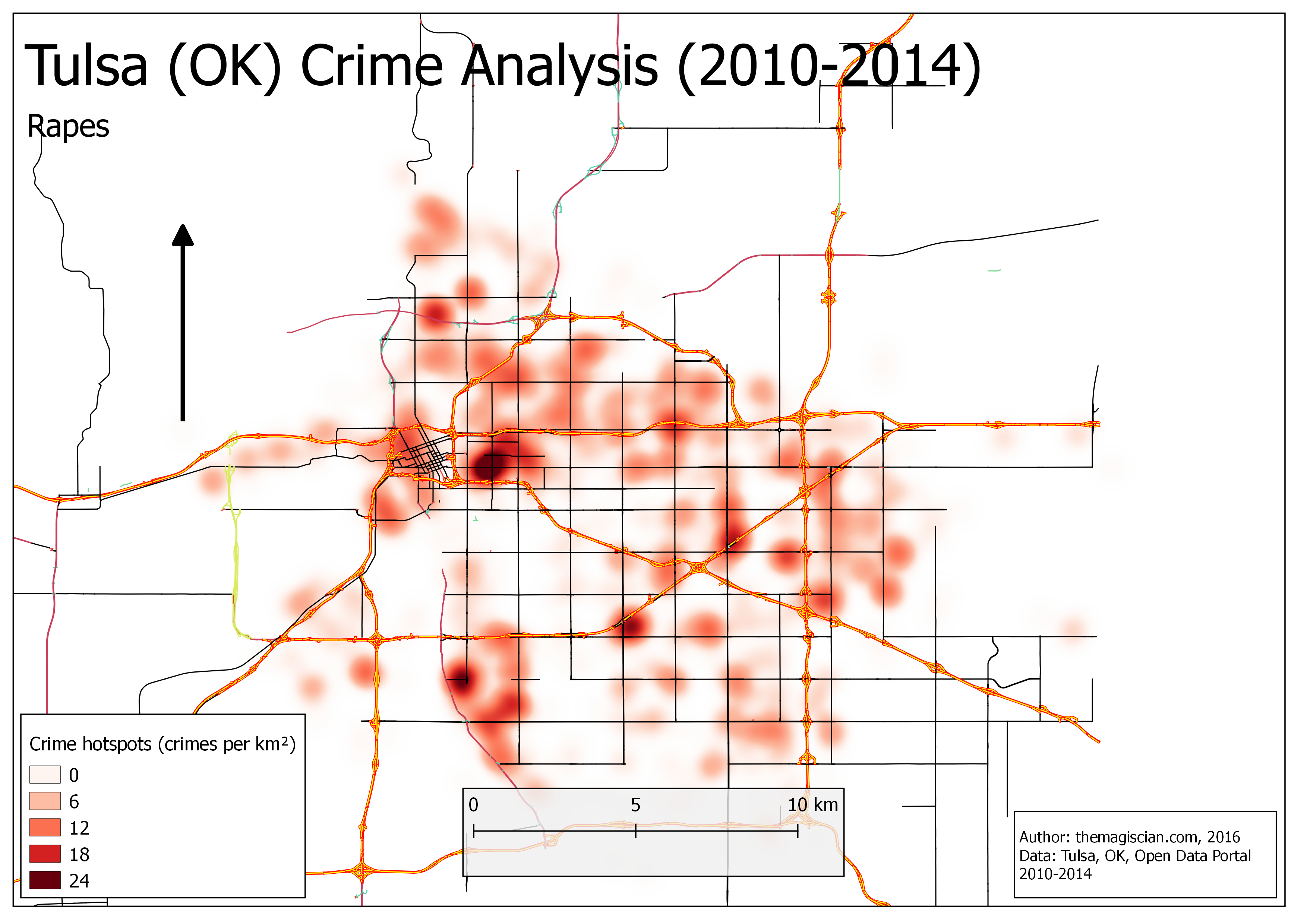
Rapes do have their biggest hotspot in the East of Downtown. We have identified a University there.

Robberies

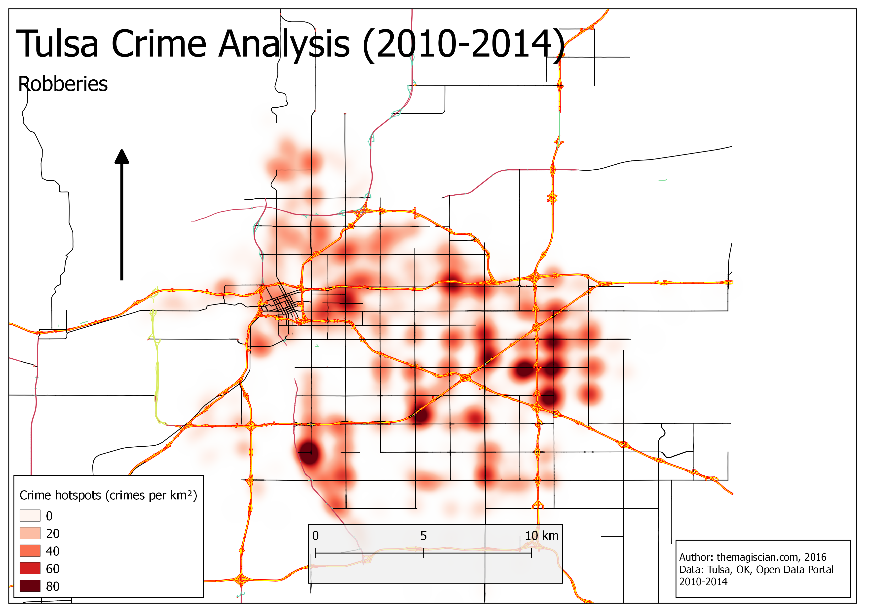
Four hotspots got our attention in the East of the City. After investigations, we noticed a lot of residential parks there.

General Crime Hotspots

As you may have noticed, some hotspots areas are the same for almost all the analysis.

Larcenies and robberies are concentrated in crowded areas (shopping malls, Downtown area, University Campuses, residential parks).

One spot seems to appears in EVERY crime type map and we did already spot a multiple shooting there: It’s the place called Fairmont Terrace Apartments (now Savannah Landings), which is a residential park. A lot of crimes do occur there as we can find statements on the internet. According to recent news, the problems have been identified and things are changing.

Per month

Are there some some months that are more prone to crimes?

-- GET TOTAL NUMBER OF CRIMES PER MONTH
SELECT EXTRACT(MONTH FROM START_DATE) month_, count(*) total_crimes FROM CRIMES GROUP BY month_ order by total_crimes desc;

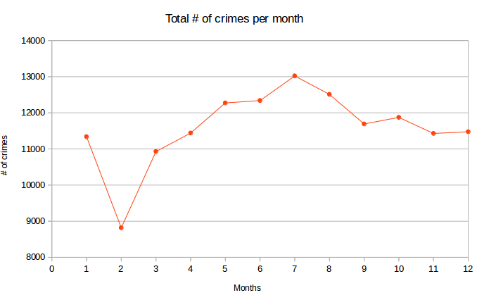
Most crimes occur during the Summer season. Is it maybe due because people are more on vacation (buglaries) ? The different statistics per crime type and month will give us the answer.

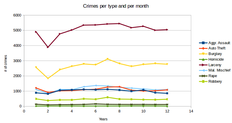
A lot of conclusions can be drawn from this chart but we can see clearly that burglaries and robberies are at their highest in the summer months. On the contrary, we see that all crime type drop significantly during the winter months, and especially in February. We make the assumptions that people are more going out in the Summer and are thus more prone to these types of crimes.

Per day

How do the crimes spread accross the week?

-- GET TOTAL NUMBER OF CRIMES PER DAY OF THE WEEK
SELECT start_day day_of_the_week, count(*) total_crimes FROM CRIMES GROUP BY day_of_the_week order by total_crimes desc;

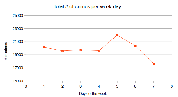
Crimes do most occurs on Fridays and Saturdays. People tend more to go out on these days of the week.

Per hour of the day

Do crimes most occur during the day or during the night?

Attention: for the hours (start_time and end_time), we noticed that there is an abnormal amount of crimes occurring at midnight and for which the start_time is the same as the end_time. Out of a total of 15 704 crimes with a duration of less than a minute, 2738 (17.44%) occur at midnight (and hence stopped at midnight as well). We decide to not take into account these data. We assume these are the default hour for crime for which the timestamps are unknown.

-- GET TOTAL NUMBER OF CRIMES PER HOUR 
SELECT EXTRACT(HOUR FROM START_TIME) hour_, count(*) total_crimes FROM CRIMES WHERE (((EXTRACT(MINUTE FROM (end_time - start_time)) + ABS(EXTRACT(hour FROM (end_time - start_time))) * 60 ) < 1) AND extract(hour from start_time) = 0) = FALSE GROUP BY hour_ order by total_crimes desc;

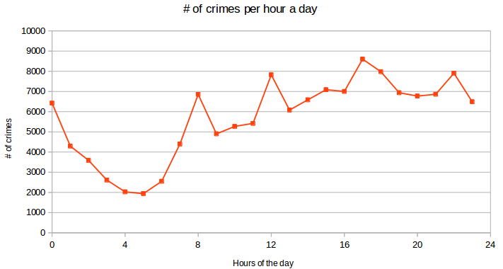
As we do not have a background in criminology, we can only do assumptions about why there’s a big gap between the morning hours et the rest of the day. One can be the following: as we’ve previously seen, most of the crimes are larcenies. These mostly occur in crowded areas such as shopping malls or streets. These are not open (or less frequented) during the night. The chart tells us that the # of crimes is increasing throughout the day to peak at 5pm.

Is it maybe due to the end of workday for most of the workers?. The peak at 12pm, is it due to the fact that people tend to go out for dinner? It the 8am peak linked to the “going to work” of the workers?

As for always, these are just assumptions and need to be verified.

Per hour a day

To fine-grain the analyses, we will analyse at which hour of which day most crimes occur.

SELECT distinct START_DAY, EXTRACT(HOUR FROM START_TIME) hour_, count(*) total_crimes FROM CRIMES WHERE ((EXTRACT(MINUTE FROM (end_time - start_time)) + ABS(EXTRACT(hour FROM (end_time - start_time))) * 60 ) < 1 AND EXTRACT(hour FROM start_time) = 0) = FALSE GROUP BY START_DAY, hour_ ORDER BY total_crimes desc LIMIT 10;

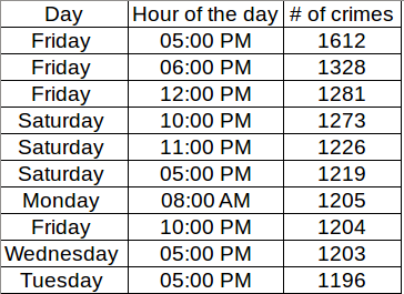
Most crimes occur Friday at the beginning of the evening (5pm then 6pm). Looking at the table, we see a tendency for crimes to occur mostly in the evening.

Per year

Are there as many crimes each year? Or are there significant variation?

First, we create the view for each year.

CREATE VIEW CRIMES_2010 AS SELECT * FROM CRIMES WHERE EXTRACT(YEAR FROM START_DATE) = 2010;
CREATE VIEW CRIMES_2011 AS SELECT * FROM CRIMES WHERE EXTRACT(YEAR FROM START_DATE) = 2011;
CREATE VIEW CRIMES_2012 AS SELECT * FROM CRIMES WHERE EXTRACT(YEAR FROM START_DATE) = 2012;
CREATE VIEW CRIMES_2013 AS SELECT * FROM CRIMES WHERE EXTRACT(YEAR FROM START_DATE) = 2013;
CREATE VIEW CRIMES_2014 AS SELECT * FROM CRIMES WHERE EXTRACT(YEAR FROM START_DATE) = 2014;

-- Count per year
SELECT count(*) FROM CRIMES_2010;
-- 28832
SELECT count(*) FROM CRIMES_2011;
-- 28871
SELECT count(*) FROM CRIMES_2012;
-- 27439
SELECT count(*) FROM CRIMES_2013;
-- 27667
SELECT count(*) FROM CRIMES_2014;
-- 26330

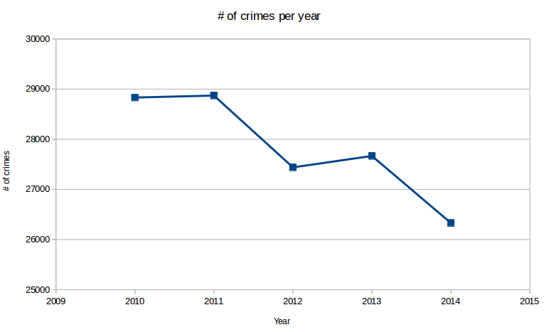
As we can see from the chart, there a significant drop in the crime numbers over the period 2010-2014 (a drop of 8.68%). Is it due to more efficient police? Of are people committing less crimes as economic situations get better?

Per crime per year

We notice a general drop in the number of crimes from 2010-2014. But which crime type did significantly drop during this period?

SELECT ucc_crime1 CRIME_TYPE, count(*) TOTAL_CRIMES_2010 FROM CRIMES_2010 GROUP BY ucc_crime1 ORDER BY TOTAL_CRIMES_2010 desc;
SELECT ucc_crime1 CRIME_TYPE, count(*) TOTAL_CRIMES_2011 FROM CRIMES_2011 GROUP BY ucc_crime1 ORDER BY TOTAL_CRIMES_2011 desc;
SELECT ucc_crime1 CRIME_TYPE, count(*) TOTAL_CRIMES_2012 FROM CRIMES_2012 GROUP BY ucc_crime1 ORDER BY TOTAL_CRIMES_2012 desc;
SELECT ucc_crime1 CRIME_TYPE, count(*) TOTAL_CRIMES_2013 FROM CRIMES_2013 GROUP BY ucc_crime1 ORDER BY TOTAL_CRIMES_2013 desc;
SELECT ucc_crime1 CRIME_TYPE, count(*) TOTAL_CRIMES_2014 FROM CRIMES_2014 GROUP BY ucc_crime1 ORDER BY TOTAL_CRIMES_2014 desc;

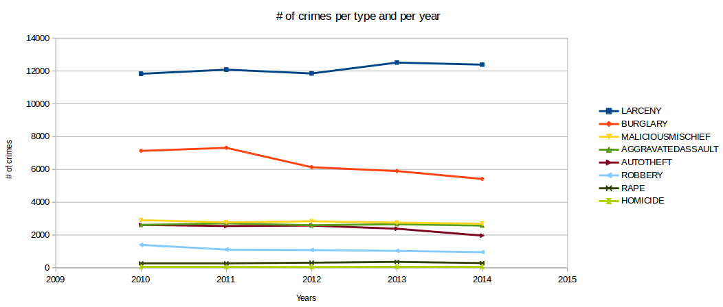
As we can see from the chart, the drop in the total number of crimes is mainly due to the drop in burglaries and Auto thefts. Larcenies, on the contrary, tend to increase.

Conclusions

A lot of conclusions can be drawn out of our analyses and we cannot cover the whole bunch of possible analyses that can be made with the provided data. We did only cover a very tiny portion of it. Also, as we have no background in criminology, our assumptions have to be verified more seriously.

GIS can anyway give some first answers to crime data analyses. The power of GIS tools resides in giving some insights on “where” question when talking about crimes.

I did not explain how I did the maps in QGIS. If you are interested, please free free to contact me!

Cheers,

Daniel

Additional Analysis

Our analyses are far from being sufficient, we’re just presenting insights. We could have added to the situational map the Arkansas River, and not just the road network.

We could also add the police stations to the map to see if there is any link with Crime Hotspot. For example: Do the Police stations prevent crimes in the areas they are situated?

The public transportation network can also be added to the map. Many crimes do occur near networks nodes because escape possibilties are multiple.

The Magiscian

Crime Data analyses (Tulsa, OK)