

Posts by themagiscian:
- Prepare the database model for storing the incoming data (PostGIS)
- Develop a script that gathers the latest positions available and updates the database (Python)
- Expose the data via an Application Server (GeoServer)
- Consume the WMS services and display the data on a map (OpenLayers)
Tracking Sydney Ferries in real time with OpenSource GIS tools
July 23rd, 2017The trend in IT is currently dominated by terms like “Big Data”, “Real-Time”, “Fast Data”, “Smart Data”, … GIS is no exception as most of the data out there can be geolocalized. As the amount of available data is growing and becoming huge, there are more and more agencies (often public) who put their data for free on Open Data Portals to crowdsource data analyses. They, in turn, become bread and butter for GIS enthusiasts for their applications.
Living in Sydney since January (I live in Melbourne now), I came across the wonderful Public Transport Open Data Portal of NSW.

Besides all the static data, there is a web API streaming the real-time position of the vehicles of the NSW Transport Company like the trains, busses, ferries, and light rails. This particular API got my attention and I was curious to exploit this API to display the ferries on a map using exclusively Open Source GIS technologies. The end product of my development looks like this (one position every 10 seconds in accelerated mode):
To reproduce at home here’s the plan
NB: All the codes can be found on my github page.
Set up the database (PostGIS)
We need at least two tables: One that welcomes the latest positions for every ferry, and another for archiving these positions.
The first step is to create the database with a superuser, to connect to it with the current user, and to create the extension.
-- Database creation
DROP DATABASE sydney_transport;
CREATE DATABASE sydney_transport WITH OWNER themagiscian;
-- Connect to the database with the correct user as we're creating the postgis extension
\c sydney_transport postgres
-- If needed, create the postgis extension
CREATE EXTENSION postgis;
Let’s create our ferries table based on the structure of the data coming from the API. We will see it more in detail later but the raw data coming from the API looks like this:
id: "3366bd10-e7be-4bee-9934-5719b8cccfd0"
vehicle {
 trip {
 trip_id: "NB164-3196"
 }
 position {
 latitude: -33.8606529236
 longitude: 151.211135864
 bearing: 177.399993896
 speed: 0.300000011921
 }
 timestamp: 1495538649
 vehicle {
 id: "1011"
 label: "Scarborough"
 }
}
Create the table with the same structure.
DROP TABLE ferries;
CREATE TABLE ferries (
 id serial NOT NULL PRIMARY KEY,
 entity_id varchar(36) NOT NULL ,
 trip_id varchar(10),
 vehicle_id varchar(4) NOT NULL ,
 label varchar(20) NOT NULL ,
 time_text varchar(24),
 time_posix integer,
 latitude double precision,
 longitude double precision,
 bearing double precision,
 speed double precision,
 geom geometry(Point, 4326)
);
Note the field time_posix: we will have to convert it to a human readable format (that’s why we create the time_text field as well). Let’s create another table with the same structure but for storing the historical values.
DROP TABLE ferries_hist;
CREATE TABLE ferries_hist (
 id serial NOT NULL PRIMARY KEY,
 entity_id varchar(36) NOT NULL ,
 trip_id varchar(10),
 vehicle_id varchar(4) NOT NULL ,
 label varchar(20) NOT NULL ,
 time_text varchar(24),
 time_posix integer,
 latitude double precision,
 longitude double precision,
 bearing double precision,
 speed double precision,
 geom geometry(Point, 4326)
);
The structure of our data model and the rules are as follows:
- Data coming from the API are inserted into the ferries table
- A trigger is fired for each bulk insert to duplicate the data into the ferries_hist table
- Both tables have a trigger that fires the geometry creation based on the longitude and latitude provided from the raw data
- The trigger on the ferries table also deletes entries so that there is only one entry per ferry with the latest position
- After every insert into the ferries and ferries_hist tables, there’s a trigger that checks and deletes for redundant entries
- As the ferries table changes quite often – every 10 seconds as we will see later – we create on top of it a VIEW
- Last but not least, we regularly update (after 50 inserts) the spatial index
The Trigger that is fired when INSERT operations are made on the ferries table updates the ferries_hist table
06.CREATE_TRIGGER_TO_HIST.sql

DROP TRIGGER sendtohist_trigger ON ferries;
DROP FUNCTION sendtohist();
CREATE OR REPLACE FUNCTION sendtohist()
RETURNS trigger
LANGUAGE plpgsql
SECURITY DEFINER
AS $BODY$
DECLARE
vid text;
BEGIN
INSERT INTO ferries_hist (entity_id, trip_id, vehicle_id, label,
time_text, time_posix, latitude, longitude, bearing, speed)
VALUES (NEW.entity_id, NEW.trip_id, NEW.vehicle_id, NEW.label,
NEW.time_text, NEW.time_posix, NEW.latitude, NEW.longitude,
NEW.bearing, NEW.speed);

RETURN NEW;
END
$BODY$;

CREATE TRIGGER sendtohist_trigger
AFTER INSERT
ON ferries
FOR EACH ROW
EXECUTE PROCEDURE sendtohist();
After each INSERT, the geometry is calculated with the provided longitude and latitude.
07.CREATE_TRIGGER_SETGEOM.sql

DROP TRIGGER setgeom_trigger ON ferries_hist;
DROP TRIGGER setgeom_trigger ON ferries;
DROP FUNCTION setgeom();
CREATE OR REPLACE FUNCTION setgeom()
RETURNS trigger
LANGUAGE plpgsql
SECURITY DEFINER
AS $BODY$
BEGIN
  EXECUTE 'UPDATE ' || TG_TABLE_NAME || ' SET geom =
  ST_SetSRID(ST_Point(longitude, latitude), 4326) WHERE geom IS NULL';
RETURN NEW;
END
$BODY$;

CREATE TRIGGER setgeom_trigger
AFTER INSERT
ON ferries_hist
FOR EACH ROW
EXECUTE PROCEDURE setgeom();

CREATE TRIGGER setgeom_trigger
AFTER INSERT
ON ferries
FOR EACH ROW
EXECUTE PROCEDURE setgeom();
The trigger that deletes the duplicates in each table.
08.CREATE_TRIGGER_DELETE_DUPLICATES.sql

DROP FUNCTION deleteduplicate();
CREATE OR REPLACE FUNCTION deleteduplicate()
RETURNS void
LANGUAGE plpgsql
AS $BODY$
DECLARE
 vid text;
BEGIN

FOR vid IN SELECT DISTINCT vehicle_id FROM ferries
 LOOP
 RAISE NOTICE 'DELETE FROM ferries WHERE vehicle_id = %
AND time_posix NOT IN (SELECT MAX(time_posix) FROM ferries
WHERE vehicle_id = %)', vid, vid;
 EXECUTE 'DELETE FROM ferries WHERE vehicle_id = '''
 || vid || ''' AND time_posix NOT IN (SELECT MAX(time_posix)
 FROM ferries WHERE vehicle_id = ''' || vid || ''')';
 END LOOP;

DELETE FROM ferries
 WHERE id NOT IN (
 SELECT MAX(f.id)
 FROM ferries As f
 GROUP BY f.vehicle_id, f.time_posix
 );

DELETE FROM ferries_hist
 WHERE id NOT IN (
 SELECT MAX(f.id)
 FROM ferries_hist As f
 GROUP BY f.vehicle_id, f.time_posix
 );
END
$BODY$;
A function that recreates the spatial index.
09.CREATE_GIST_INDEX.sql
DROP FUNCTION createGistIndex(VARCHAR);
CREATE OR REPLACE FUNCTION createGistIndex(table2Index VARCHAR)
RETURNS void
LANGUAGE plpgsql
AS $BODY$
DECLARE
 t2i varchar := replace(table2Index, '"', '');
BEGIN
 EXECUTE 'DROP INDEX IF EXISTS ' || t2i || '_gix;';
 EXECUTE 'CREATE INDEX ' || t2i || '_gix ON ' || t2i || ' USING GIST (geom);';
END
$BODY$;
That’s it for the database part!
Get the real-time positions and insert them into a database (Python)
This is the core of our application: get the real-time data and insert them into our database. The data format distributed through the api is the GTFS-realtime format. This format stands for “General Transit Feed Specification” and is an open data format for public transportation-related information. This format is based on Protocol buffers which are a “language-neutral, platform-neutral extensible mechanism for serializing structured data” according to Google.
The link to access the web API is the following https://opendata.transport.nsw.gov.au/dataset/public-transport-realtime-vehicle-positions. Note that you have to create an account to have access to the data.
There are tons of technologies out there for handling GTFS-realtime data. We opt for the versatile Python language for its simplicity of implementation.
Let’s start with the imports.
from google.transit import gtfs_realtime_pb2
from psycopg2 import sql
import urllib2
import time
import psycopg2
import threading
We need the google.transit package in order to be able to read the encrypted real-time data coming from the API. psycopg2 is for the connection to the database, urllib2 is for sending our request to the API.
We then defined our global database variables to open a connection to the database. After that, we define a feed object that will unwrap the encrypted response coming from the API. Finally, we set the HTTP Get parameters to be sent to the API.
try:
 connection = psycopg2.connect(host=hostname, user=username, password=password, dbname=database)
 feed = gtfs_realtime_pb2.FeedMessage()
 req = urllib2.Request('https://api.transport.nsw.gov.au/v1/gtfs/vehiclepos/' + transport)
 req.add_header('Accept', 'application/x-google-protobuf')
 req.add_header('Authorization', 'apikey ***')
except e:
 print e
Note that we use the “transport” variable which takes here the String value “ferries”. This one can be changed to “trains”, “buses”, or “light rail.” Not to forget to create a function that will actually execute our database queries once the information from the API is gathered.
def doQuery(conn, query, data):
 cur = conn.cursor()
 cur.execute(query, data)
Now comes the core of our script:
- Gather the response from the API,
- putting the results in a template INSERT INTO database request,
- and executing these request to the database
All these operations are executed every, let’s say, 10 seconds – and thus the use of the thread in the script that follows.
The function to be executed every 10 seconds is obviously called getPositions()
def getPositions():
 global COUNT
 threading.Timer(10.0, getPositions).start()
 response = urllib2.urlopen(req)
 feed.ParseFromString(response.read())
 doQuery(connection, """BEGIN""", None)
The parameter “response” contains the whole response from the API. The first “commit” operation start the whole database transaction. Transaction is very important here: For each query to the API, there is a big bunch of data retrieved and they need to be processed and inserted into the database. The “ParseFromString” operation cuts the response into smaller pieces and each piece is put into an array we exploit later in a for loop.
for entity in feed.entity:
 query = "INSERT INTO {} (entity_id, trip_id, vehicle_id, label, time_text, time_posix, latitude, longitude, bearing,
speed) VALUES (%s, %s, %s, %s, %s, %s, %s, %s, %s, %s);"
 data = (str(entity.id), str(entity.vehicle.trip.trip_id), str(entity.vehicle.vehicle.id),
  str(entity.vehicle.vehicle.label), str(time.ctime(int(entity.vehicle.timestamp))), str(entity.vehicle.timestamp),
  str(entity.vehicle.position.latitude), str(entity.vehicle.position.longitude), str(entity.vehicle.position.bearing),
  str(entity.vehicle.position.speed))
 doQuery(connection, sql.SQL(query).format(sql.Identifier(transport)), data)
 doQuery(connection, "SELECT deleteduplicate();", None)
 doQuery(connection, sql.SQL("SELECT createGistIndex('{}');").format(sql.Identifier(transport)), None)
The separation between the query template and the data to be inserted in, as preconized by psycopg2, is respected here. The whole is then sent to the doQuery function we discussed earlier.
The whole script is then run and as said, it gather new data every 10 seconds and feeds the database.
Here’s a sample of the results we got.
 id     | trip_id    | label          | time_text                | latitude| longitude|bearing | speed
--------+------------+----------------+--------------------------+---------+---------+---------+-------
1874191 | ES170-2960 | Mary MacKillop | Wed May 03 22:15:08 2017 | -33.855 | 151.188 | 330.800 | 0.100
1874195 | ML172-2846 | Freshwater     | Wed May 03 22:15:08 2017 | -33.860 | 151.211 | 104.5   | 0
1874197 | MS160-3114 | Golden Grove   | Wed May 03 22:15:09 2017 | -33.842 | 151.232 | 334.800 | 5.400
1874203 | NB162-3116 | Friendship     | Wed May 03 22:15:09 2017 | -33.860 | 151.211 | 35.800  | 0.100
1874205 | NB164-3116 | Fishburn       | Wed May 03 22:15:09 2017 | -33.851 | 151.211 | 293.200 | 11.500
1874206 | RV230-3080 | Betty Cuthbert | Wed May 03 22:15:09 2017 | -33.854 | 151.187 | 148.300 | 0
1874208 | RV236-3080 | Marjorie Jackson|Wed May 03 22:15:09 2017 | -33.842 | 151.180 | 132.100 | 5.400
 864505 | ES644-2832 | Susie O'Neill  | Sun Apr 30 16:49:09 2017 | -33.855 | 151.188 | 68.600  | 0
 884575 | TZ650-3078 | Lady Herron    | Sun Apr 30 17:33:13 2017 | -33.860 | 151.210 | 190.500 | 2.600
1856440 | DH156-2800 | Louise Sauvage | Wed May 03 20:28:07 2017 | -33.850 | 151.214 | 331.600 | 6.010
Expose the data via an Application Server (GeoServer)
In our n-tier architecture, our cartographic server is GeoServer, which is a reliable Open Source product for our purpose.
We just create a layer on top of the view we defined during the database part.
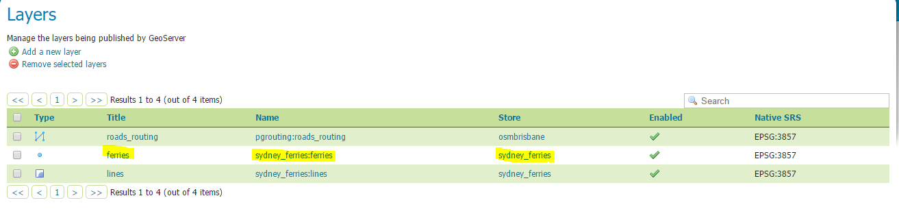
Consume the WMS service and display the data on a map (OpenLayers)
Beside all the conventional files (index.html, style.css, etc.) the most interesting file is add_sflayer.js. We reference the layer and add it to the map.
var params_ferries = {'LAYERS': 'sydney_ferries:ferries'}
var wmsSource_ferries = new ol.source.TileWMS({
 url: 'http://jupiter:8080/geoserver/sydney_ferries/wms',
 params: params_ferries
})

var wmsLayer_ferries = new ol.layer.Tile({
 source: wmsSource_ferries
});
For having a dynamic map, or in other words to see the ferries moving on the map, we need to refresh the view at specified intervals. We use the same 10 seconds as we defined for the Python script.
var refreshLayer = function(){
 wmsSource_ferries.updateParams({"time": Date.now()});
 updateTimer = setTimeout(function() {
 refreshLayer();
 }, 10000);
}

refreshLayer();
It reads again the WMS source, whose data are coming from the ferries_view. Just to remind, this view is on top of the ferries table, which is refreshed every 10 seconds.
Bonus
After a while, there are sufficient data into the database to create traces for the ferries. Just link all the points of the same ferries together to get the path as highlighted in blue in the previous screenshot.
CREATE TABLE lines AS
SELECT fh.vehicle_id, fh.label, ST_LineToCurve(ST_MakeLine(fh.geom ORDER BY time_posix)) geom
 FROM ferries_hist fh GROUP BY fh.vehicle_id, fh.label;
CREATE INDEX lines_gix ON lines USING GIST (geom);
VACUUM ANALYZE lines;
Statistics
The script ran the whole day on Wednesday the 3rd of May from 06:49:07 to 22:15:09. During that period, 129 446 positions have been gathered for the 20 ferries composing the fleet., and which are Alexander, Betty Cuthbert, Charlotte, Dawn Fraser, Fishburn, Freshwater, Friendship, Golden Grove, Lady Herron, Lady Northcott, Louise Sauvage, Marjorie Jackson, Mary MacKillop, Nicole Livingstone, Pam Burridge, Scarborough, Sirius, SuperCat 4, Supply, and Susie O’Neill.
The 3 ferries that travelled the longest distances during that day are the following ones:
select vehicle_id, label, st_length(geom::geography)/1000 "distance (km)" from lines_0305 order by length desc;
 vehicle_id | label            | distance (km)
------------+------------------+------------------
 1020       | Marjorie Jackson | 242.693213184936
 1002       | Freshwater       | 209.724200233982
 1027       | SuperCat 4       | 200.775006102889
The first one is the Parramatta line, the second is the Manly line, and the third covers the Eastern Suburbs.
Cheers,
Daniel
Winter solstice and Hillshade over Brussels
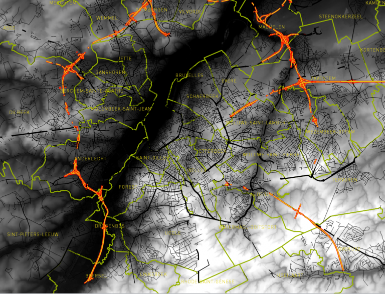
December 22nd, 2016Yesterday, the 21st of December 2016, was the shortest day in the Northern Hemisphere. In other words, it is the day the sun is the lowest in the sky at noon of all the year. This winter solstice gave me the idea to create a series of hillshade of Brussels to show how the illumination change throughout the day, every 30 minutes, from sunrise to sunset. The result is the following time series in a modelling clay-like terrain.
The Hillshades shown in the time series were created using a DEM and PostGIS. The visualization is done using QGIS.
Technical Recipe
DEM
We’re starting with the same DEM we used in a previous article.
What are the sun’s azimuth and elevation at each hour of the day?
For knowing that, we use the http://www.sunearthtools.com/ website, which give us for Brussels on the 21st of December 2016.
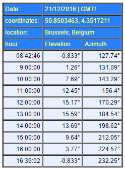
Create the hillshades
The DEM is imported into a PostGIS database. There’s a special function within PostGIS for creating Hillshades. It is called ST_Hillshade. Using the Elevation and Azimuth values shown above, we generated a series of functions for showing the hillshade each 30 minutes, from sunrise to sunset.
DROP TABLE IF EXISTS hill_074246;
CREATE TABLE hill_074214 AS SELECT ST_HillShade(rast, 1, '8BUI', 127.74, 0, 255, 1.0, TRUE) rast
FROM brussels_dem_10m;
ALTER TABLE hill_074214 ADD COLUMN rid serial;
ALTER TABLE hill_074214 ADD CONSTRAINT hill_074214_pk PRIMARY KEY (rid);
CREATE INDEX hill_074214_gix ON hill_074214 USING GIST (st_convexhull (rast ) );
DROP TABLE IF EXISTS hill_080000;
CREATE TABLE hill_080000 AS SELECT ST_HillShade(rast, 1, '8BUI', 131.09, 1.26, 255, 1.0, TRUE) rast
FROM brussels_dem_10m;
ALTER TABLE hill_080000 ADD COLUMN rid serial;
ALTER TABLE hill_080000 ADD CONSTRAINT hill_080000_pk PRIMARY KEY (rid);
CREATE INDEX hill_080000_gix ON hill_080000 USING GIST (st_convexhull (rast ) );
[...]
Note: The hours used in the script are in UTC while those from the table are in local time.
For the visualization in QGIS, we used a reverse greyscale: lowest values are in white while highest values are in black. If we do not do so, the modelling clay aspect of the terrain would seem like reversed: ridge lines look like valleys and valleys look like ridge lines.
Observations
Looking attentively to the variations in illumination throughout the day, we can observe how the angle of the incoming light plays on the shadow directions. This is especially true for the river system in the South East part of the scene.
Conclusions
With a DEM of the city of Brussels, with tools such as PostGIS and QGIS and with an ephemeris table, it is possible to create a series of Hillshade images showing the variation of the illumination every 30 minutes over the city of Brussels.
Cheers,
Daniel
Sentinel-2’s response to Trump’s Election
December 8th, 2016It couldn’t be more clear from the Sentinel-2’s side. Take a look at the following image, which was taken the 7th of November 2016, just one day before Trump’s election.
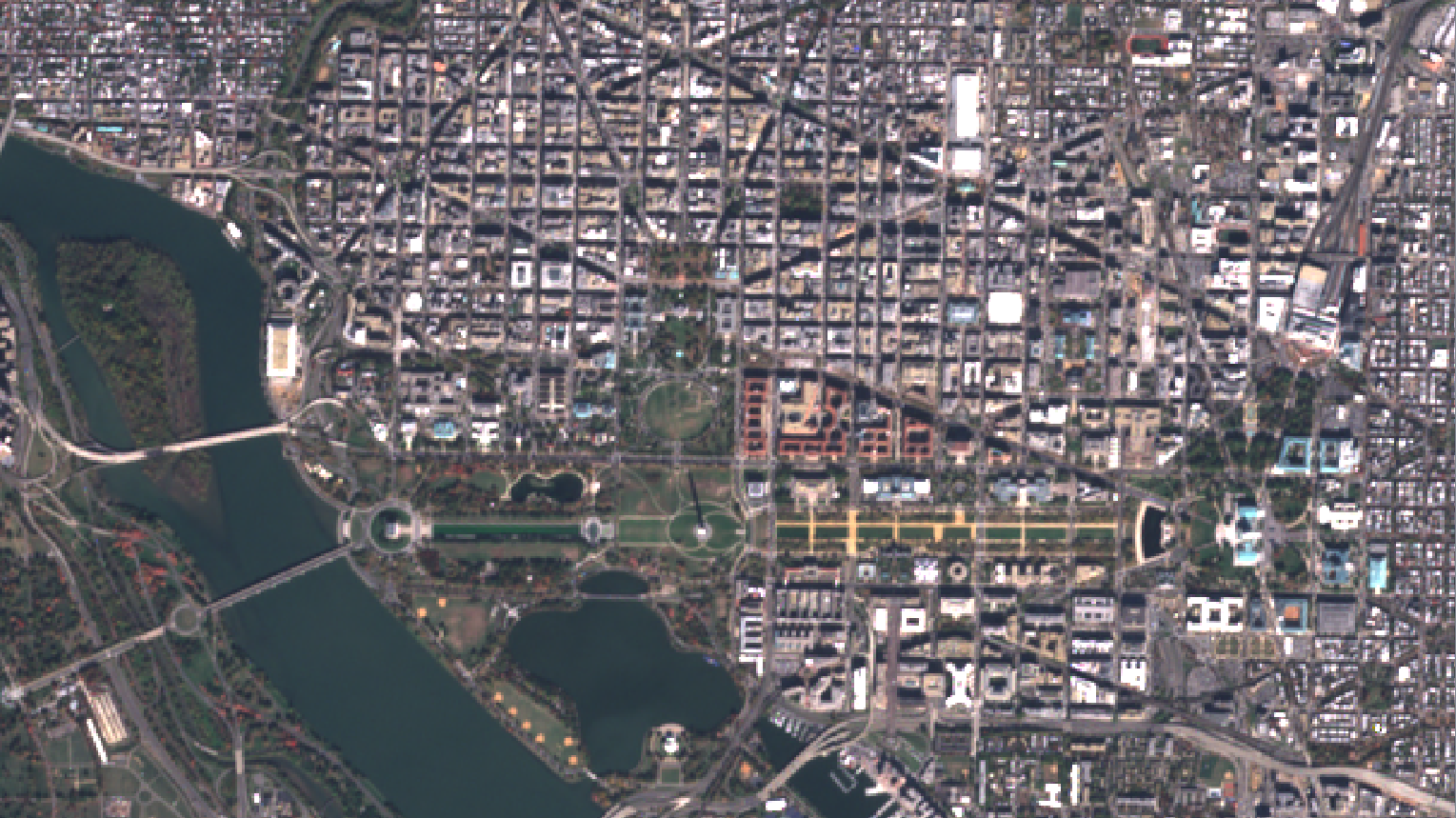
A beautiful bright sky letting the Earth uncovered for the satellite’s eyes. Right in the middle, you can spot the famous White House, the new home of Mister Trump. The West-to-East green park is the National Mall Park with the Washington Monument in the middle throwing its long shadow to the North. It currently points to the Ellipse just in the North. The small circle just above is the White House South Lawn. Trump’s new home is just further North.
Let’s see what Sentinel-2 has reserved for the after-Obama era…
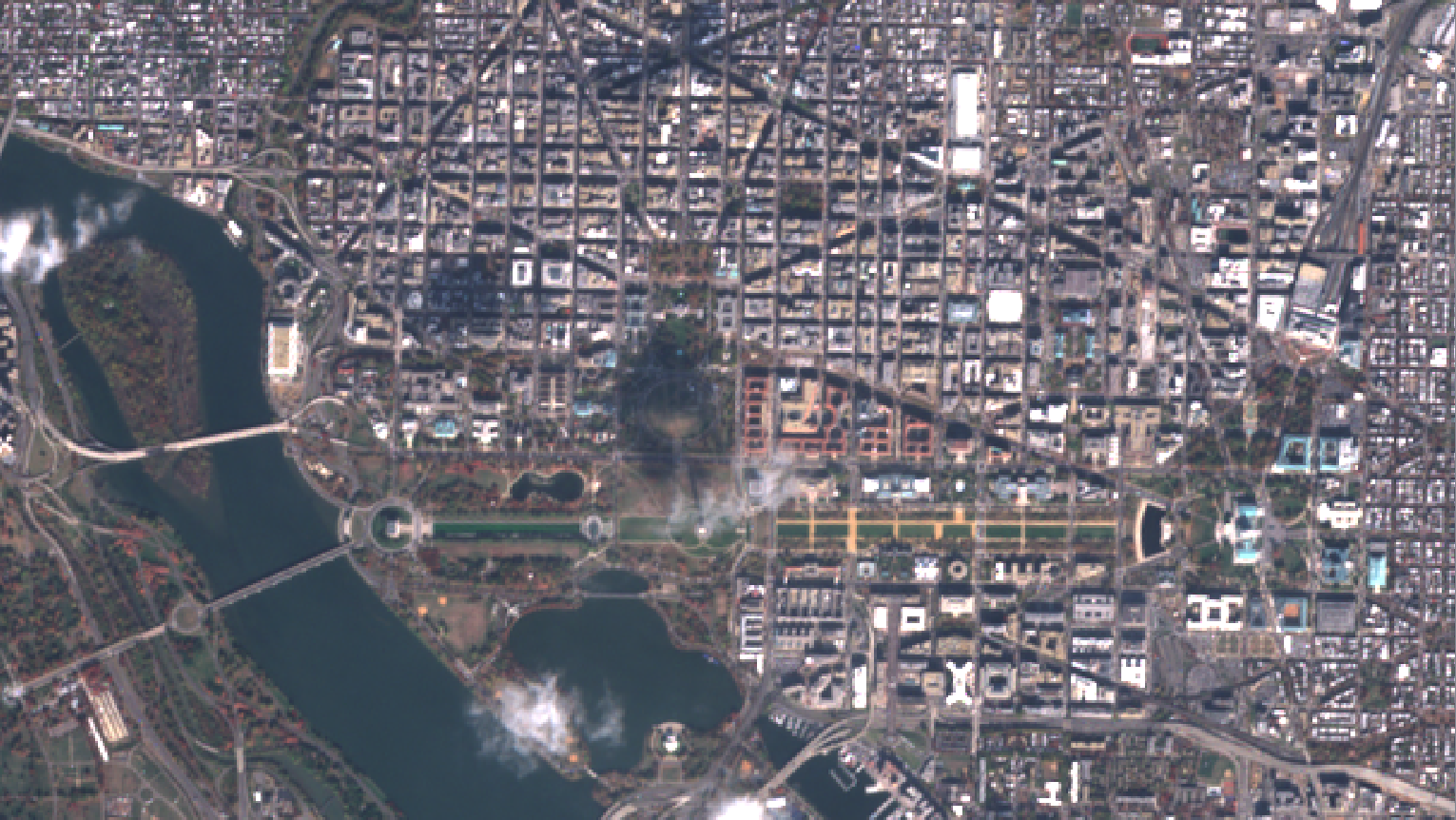
Here we have it! A big fat shadow thrown from a very small cloud (sounds familiar?). This image was taken the 17th of November, so after the election. Things are getting dark now and it seems that the Sentinel-2 satellite wants to give us a message …
And BAM!
The Sentinel-2 satellite is just more than just an amount of steel travelling at fast pace around Earth and taking pictures. He can expressed his feelings by customizing the pictures it takes from outer space. Here is the truth of the Sentinel-2 soul 🙂
Cheers,
Daniel
DEM for Slope calculations in Bicycle Routing: PostGIS
November 28th, 2016Everyone who went cycling in Belgium knows that the famous quote from Jacques Brel “Le plat pays qui est le mien” is far from being true! Belgium is globally a flat land with the highest point sitting at 694m above sea level, this is true, but once on a bike you notice immediately that painfull slopes are just around the corners. Taking into account the elevation and the slopes is important in routing algorithms.
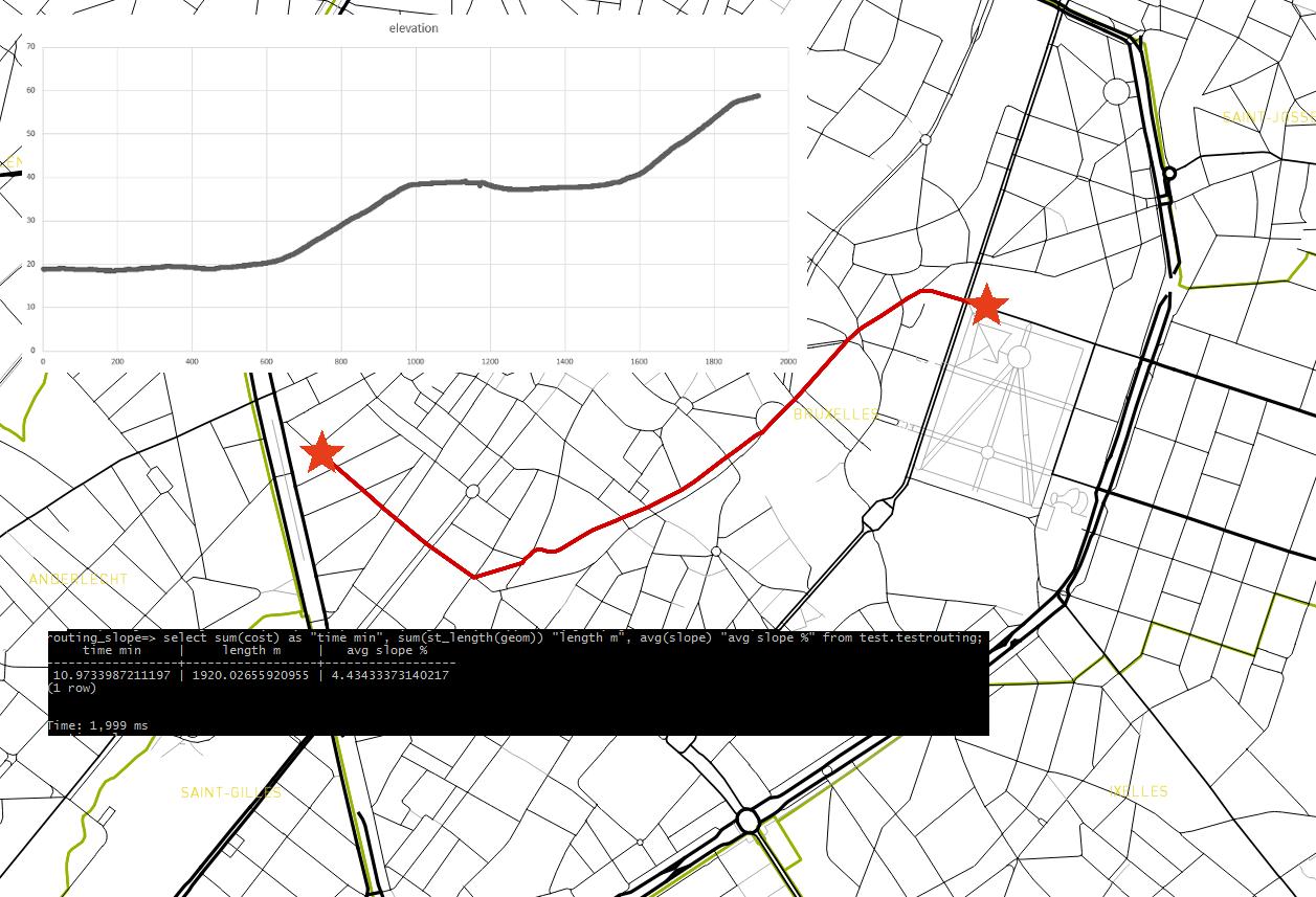
In this article, we will analyze the shortest cycling routes in Brussels by taking into account the slopes. Elderly people who wants to visit our Belgian Capital City by bike would be interested in such a map to choose going from A to B by the route offering the smallest slopes. In the following screenshot, we follow a bike going from the Bodeghem quarter to Rue de la Loi where the highest Belgian Institutions are located. The journey takes about 10 min by bike and is 1920 meters long. In the longitudinal profile, we see where the slopes are located and the elevation goes from 20m at the start to 60m at the arrival.
Routing with slope
For our exercice, with need two set of data: A DEM covering Brussels and the road network. Notice that the tools we use are PostGIS and QGIS for visualizing the results.
DATA
The DEM of 1 m resolution is coming from the agiv.be website. A real treasure having a DEM of 1m resolution in XY and 1mm in Z! Our network data comes from OpenStreetMap.
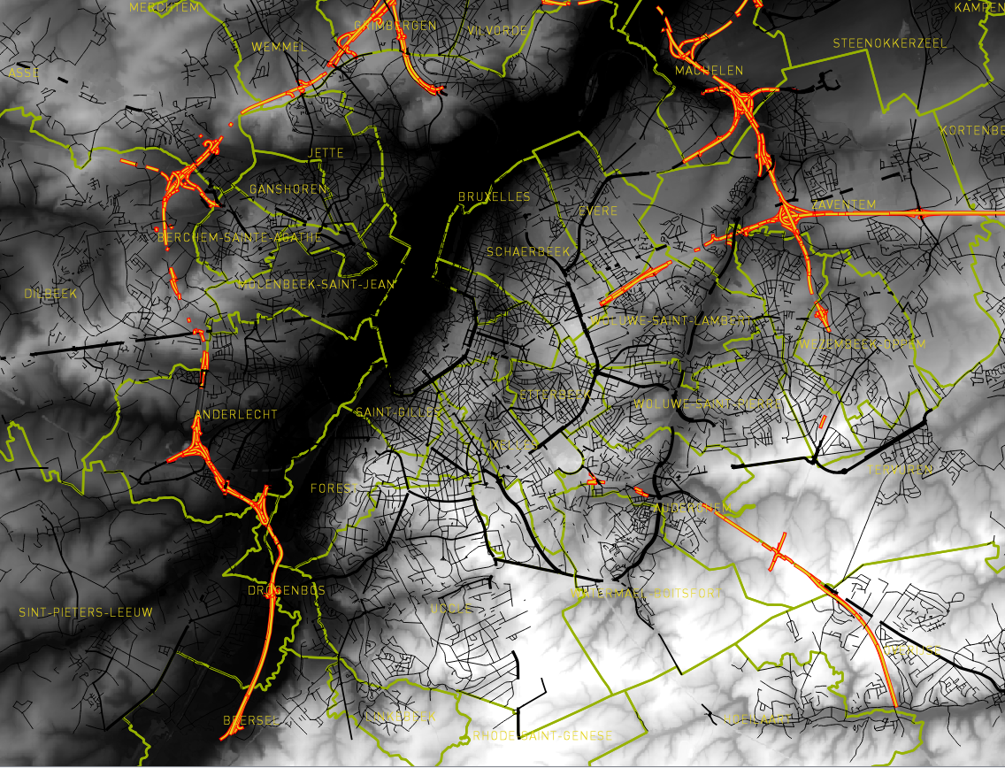
DEM and OSM
Database preparation
As always in our articles, we detail the steps to setup the environment.
Connect to PostgreSQL and create the database.
psql -Upostgres -h<ip>
CREATE DATABASE routing_slope WITH OWNER themagiscian;
Connect to the database in order to activate the extensions
\c routing_slope
CREATE EXTENSION postgis;
CREATE EXTENSION hstore;
CREATE EXTENSION pgrouting;
Connect then to the database with your user
\c routing_slope themagiscian
Data import
Our database is up and ready. Let’s import our data!
The DEM is imported using the raster2pgsql tool.
raster2pgsql -c -C -s 31370 -f rast -F -I -M -t 100x100 DHMVIIDTMRAS1m_k31.tif public.brussels_dem
| psql -Uthemagiscian -h<ip> -drouting_slope
If you did not already download the OSM data from Brussels, here is the snippet to do so, provided you have wget installed.
wget --progress=dot:mega -O "brussels2.osm"
"http://www.overpass-api.de/api/xapi?*[bbox=4.20914,50.766,4.5401,50.93593][@meta]"
From there, import the dataset into the database.
osm2pgsql -d routing_slope -H <ip> -U themagiscian -P 5432 -W -S default.style --hstore brussels.osm
Database cleaning
Our imports created a lot of stuff in our database. Here we’re cleaning things up.
osm2pgsql assigns names to the tables. We make them more user friendly.
ALTER TABLE planet_osm_line RENAME TO streets;
All the tables we do not need are thrown away.
DROP TABLE planet_osm_nodes;
DROP TABLE planet_osm_point;
DROP TABLE planet_osm_polygon;
DROP TABLE planet_osm_rels;
DROP TABLE planet_osm_roads;
DROP TABLE planet_osm_ways;
We used to name the geomety column ‘geom’
ALTER TABLE streets RENAME way TO geom;
As OSM comes with a tremendous amount of columns we do not need, we decide also to throw away all the fields we do not need.
ALTER TABLE streets DROP COLUMN access, DROP COLUMN "addr:housename", DROP COLUMN "addr:housenumber",
DROP COLUMN "addr:interpolation", DROP COLUMN admin_level, DROP COLUMN aerialway, DROP COLUMN aeroway,
DROP COLUMN amenity, DROP COLUMN area, DROP COLUMN barrier, DROP COLUMN brand, DROP COLUMN boundary,
DROP COLUMN building, DROP COLUMN construction, DROP COLUMN covered, DROP COLUMN culvert, DROP COLUMN cutting,
DROP COLUMN denomination, DROP COLUMN disused, DROP COLUMN embankment, DROP COLUMN foot,
DROP COLUMN "generator:source", DROP COLUMN harbour, DROP COLUMN historic, DROP COLUMN horse,
DROP COLUMN intermittent, DROP COLUMN junction, DROP COLUMN landuse, DROP COLUMN layer, DROP COLUMN leisure,
DROP COLUMN lock, DROP COLUMN man_made, DROP COLUMN military, DROP COLUMN motorcar, DROP COLUMN name,
DROP COLUMN "natural", DROP COLUMN office, DROP COLUMN operator, DROP COLUMN place, DROP COLUMN population,
DROP COLUMN power, DROP COLUMN power_source, DROP COLUMN public_transport, DROP COLUMN railway, DROP COLUMN ref,
DROP COLUMN religion, DROP COLUMN route, DROP COLUMN service, DROP COLUMN shop, DROP COLUMN sport,
DROP COLUMN surface, DROP COLUMN toll, DROP COLUMN tourism, DROP COLUMN "tower:type", DROP COLUMN tracktype,
DROP COLUMN water, DROP COLUMN waterway, DROP COLUMN wetland, DROP COLUMN width, DROP COLUMN wood,
DROP COLUMN z_order, DROP COLUMN way_area;
That’s all for the cleaning.
Combine Slope and Elevation Data with the Streets
That’s a tough part: Our DEM contains the elevation data and our streets are the basis of the network. Furthermore, we need to extract the slopes from the DEM and assign these values to the street segments. A lot of processing work for the computer and it is therefore important to optimize the requests in order to make processing times quicker.
First things first, we create a staging schema where we will stuff all our data and intermediary data.
CREATE SCHEMA staging;
The first step is to create a dem table of the area. In other words, we only consider pixel data on the Brussels Region
CREATE TABLE staging.brussels_dem_intersect AS
SELECT DISTINCT b.rid, b.rast rast
FROM brussels_dem b, pentagon p
WHERE ST_Intersects(b.rast, ST_Transform(p.geom,31370));
The Slopes are extracted from the DEM using the ST_Slope function.
CREATE TABLE staging.brussels_slope AS SELECT ST_Slope(b.rast, 1, '32BF', 'PERCENT', 1.0) rast FROM brussels_dem b;
ALTER TABLE staging.brussels_slope ADD COLUMN rid SERIAL PRIMARY KEY;
CREATE INDEX staging_brussels_slope_gix ON staging.brussels_slope USING GIST(st_convexhull(rast));
The ST_Slope takes as argument the raster field, the band number, the data encoding and the vertical exaggeration. The output data has to be indexed.
Our next tactic is to vectorize the Slope dataset. In other words, the pixels becomes squares and keep their slope values. You see it coming, we will in a later step extract these slope information with an intersection with the street layer.
Here’s the vectorization of the Slope dataset.
CREATE TABLE staging.brussels_slope_vector_square AS SELECT (ST_DumpAsPolygons(bslope.rast)).val slope,
(ST_DumpAsPolygons(bslope.rast)).geom geom FROM staging.brussels_slope bslope;
ALTER TABLE staging.brussels_slope_vector_square ADD COLUMN id SERIAL PRIMARY KEY;
CREATE INDEX staging_brussels_slope_vector_square_gix ON staging.brussels_slope_vector_square USING GIST(geom);
We do exactly the same with our original DEM.
CREATE TABLE staging.brussels_dem_vector_square AS SELECT (ST_DumpAsPolygons(b.rast)).val elevation,
(ST_DumpAsPolygons(b.rast)).geom geom FROM staging.brussels_dem_intersect b;
ALTER TABLE staging.brussels_dem_vector_square ADD COLUMN id SERIAL PRIMARY KEY;
CREATE INDEX brussels_dem_vector_square_gix ON staging.brussels_dem_vector_square USING GIST(geom);
Now we can intersect the vector layers and grab the Slope information to put them into the Streets layer. Notice that we cut each Streets line at the intersection. As the resolution of our Slope dataset is 1m in XY, our line will be cut in the order. Each small piece of street will have a different Slope value. A BIG AMOUNT OF STREETS PARTS WE’RE CREATING!
CREATE TABLE staging.streets_slope AS SELECT s.osm_id, bslopev.slope, belevv.elevation,
ST_Intersection(ST_Transform(s.geom, 31370), bslopev.geom) AS geom FROM streets s,
staging.brussels_slope_vector_square bslopev, staging.brussels_dem_vector_square belevv
WHERE ST_Intersects(ST_Transform(s.geom, 31370), bslopev.geom)
AND ST_Intersects(ST_Transform(s.geom, 31370), belevv.geom);
ALTER TABLE staging.streets_slope ADD COLUMN id SERIAL PRIMARY KEY;
CREATE INDEX staging_streets_slope_gix ON staging.brussels_slope_vector_square USING GIST(geom);
Notice that we make several times use of the ST_Transform function. This is mandatory because our datasets are in different SRS. Our DEM is in 31370 (Belgian Lambert 72) and the Streets from OpenStreetMap are in 3857. For the intersection function to work, both have to be in the same SRS. For you information, this takes the longest processing time. Be patient.
Our next steps is to add the Elevation information to the already cut in small pieces Streets layer.
ALTER TABLE staging.streets_slope ADD COLUMN elevation double precision;
UPDATE staging.streets_slope ss SET elevation = bdem.elevation FROM staging.brussels_dem_vector_square bdem
WHERE ST_Intersects(ST_Transform(ss.geom, 31370), bdem.geom);
UPDATE stagingt.streets_slope ss SET elevation = bdem.elevation FROM stagingt.brussels_dem_vector_square bdem
WHERE (ss.id = 92084) AND ST_Intersects(ST_Transform(ss.geom, 31370), bdem.geom);
We do add the information by adding a new field and filling it with data coming from our vectorized DEM.
Create Network
Our Streets layer is ready to be used!
We need, first, to add new columns to our Streets layer. These columns will receive the ids of both boundary points. The source and target point of the line.
ALTER TABLE staging.streets_slope ADD COLUMN "source" integer;
ALTER TABLE staging.streets_slope ADD COLUMN "target" integer;
CREATE INDEX staging_streets_slope_idx ON staging.streets_slope(id);
From there, we create the topology using the pgr_createTopology function.
SELECT pgr_createTopology('staging.streets_slope', 0.0000001, 'geom', 'id');
CREATE INDEX staging_streets_slope_source_idx ON staging.streets_slope("source");
CREATE INDEX staging_streets_slope_target_idx ON staging.streets_slope("target");
The cost of our streets, that mean, the constraint used to calculate the shortest routes, is decided to be the time, in minutes, it takes to cross it.
ALTER TABLE staging.streets_slope ADD COLUMN time_min double precision;
We arbitrary decide that a bike rides at 15km/h when it is flat. This speed goes linearily down to 5 km/h at a slope of 10%. Here are the formulae to fill these fields.
UPDATE staging.streets_slope SET time_min = (ST_Length(geom) / ((-1 * slope + 15) * 1000 / 60)) WHERE slope <= 10;
UPDATE staging.streets_slope SET time_min = (ST_Length(geom) / (5 * 1000 / 60)) WHERE slope > 10;
ALTER TABLE staging.streets_slope ADD COLUMN reverse_time_min double precision;
UPDATE staging.streets_slope SET reverse_time_min = time_min;
ALTER TABLE streets_slope_vertices_pgr SET SCHEMA staging;
ALTER TABLE staging.streets_slope_vertices_pgr RENAME the_geom TO geom;
Notice how we do aesthetics by putting the streets_slope_vertices back to the staging schema and the by default naming ‘the_geom’ becomes ‘geom’.
As we already did it in a previous article about the routing in Brisbane, we defined a wrapper function that makes it possible to calculate the least costing route from A to B. This wrapper function takes as input the x and y from the start and arrival points. From there, it chooses the corresponding nodes in the built network and calculates the lest costing route using the famous and the never out of fashion Dijkstra algorithm.
CREATE OR REPLACE FUNCTION pgr_fromAtoB(
 IN tbl varchar,
 IN x1 double precision,
 IN y1 double precision,
 IN x2 double precision,
 IN y2 double precision,
 OUT seq integer,
 OUT id integer,
 OUT name text,
 OUT heading double precision,
 OUT cost double precision,
 OUT geom geometry
 )
 RETURNS SETOF record AS
 $BODY$
 DECLARE
 sql text;
 rec record;
 source integer;
 target integer;
 point integer;

BEGIN
 -- Find nearest node
 EXECUTE 'SELECT id::integer FROM staging.streets_slope_vertices_pgr
 ORDER BY geom <-> ST_Transform(ST_GeometryFromText(''POINT('
 || x1 || ' ' || y1 || ')'',4326), 31370) LIMIT 1' INTO rec;
 source := rec.id;

EXECUTE 'SELECT id::integer FROM staging.streets_slope_vertices_pgr
 ORDER BY geom <-> ST_Transform(ST_GeometryFromText(''POINT('
 || x2 || ' ' || y2 || ')'',4326), 31370) LIMIT 1' INTO rec;
 target := rec.id;

-- Shorstaging path query (TODO: limit extent by BBOX)
 seq := 0;
 sql := 'SELECT id, geom, osm_id::text AS name, cost, reverse_time_min, source, target,
 ST_Reverse(geom) AS flip_geom FROM ' ||
 'pgr_dijkstra(''SELECT id, source::int, target::int, '
 || 'time_min::float AS cost, reverse_time_min::float AS reverse_cost FROM '
 || (tbl) || ''', '
 || source || ', ' || target
 || ' , false, true), '
 || (tbl) || ' WHERE id2 = id ORDER BY seq';

-- Remember start point
 point := source;

FOR rec IN EXECUTE sql
 LOOP
 -- Flip geometry (if required)
 IF ( point != rec.source ) THEN
 rec.geom := rec.flip_geom;
 point := rec.source;
 ELSE
 point := rec.target;
 END IF;

-- Calculate heading (simplified)
 EXECUTE 'SELECT degrees( ST_Azimuth(
 ST_StartPoint(''' || rec.geom::text || '''),
 ST_EndPoint(''' || rec.geom::text || ''') ) )'
 INTO heading;

-- Return record
 seq := seq + 1;
 id := rec.id;
 name := rec.name;
 cost := rec.cost;
 geom := rec.geom;
 RETURN NEXT;
 END LOOP;
 RETURN;
 END;
 $BODY$
 LANGUAGE 'plpgsql' VOLATILE STRICT;
The cost we defined is the time_min, the time it takes to cross each Streets segment in minutes.
Test the Routing environment!
The last and funniest part is testing out our infrastructure! From QGIS, we gather the long/lat coordinate from our points of interesting and stuff it into our wrapper function!
DROP TABLE staging.stagingrouting;
CREATE TABLE staging.stagingrouting AS SELECT p.seq, p.id, p.name, p.heading, p.cost, s.slope, s.elevation, p.geom
FROM pgr_fromAtoB('staging.streets_slope',4.34260,50.84224,4.35268,50.85145) p JOIN staging.streets_slope s ON p.id=s.id;
The following query gives us more details about the route the algorithm chose.
select sum(cost) as "time min", sum(st_length(geom)) "length m", avg(slope) "avg slope %" from test.testrouting;

 time min | length m | avg slope %
------------------+------------------+------------------
 10.9733987211197 | 1920.02655920955 | 4.43433373140217
(1 row)
Important to notice: the average slope is not quite correct. To have the average slope, we need to ponderate each Streets segment with its length. Here it is only an arithmetic average, which is not correct.
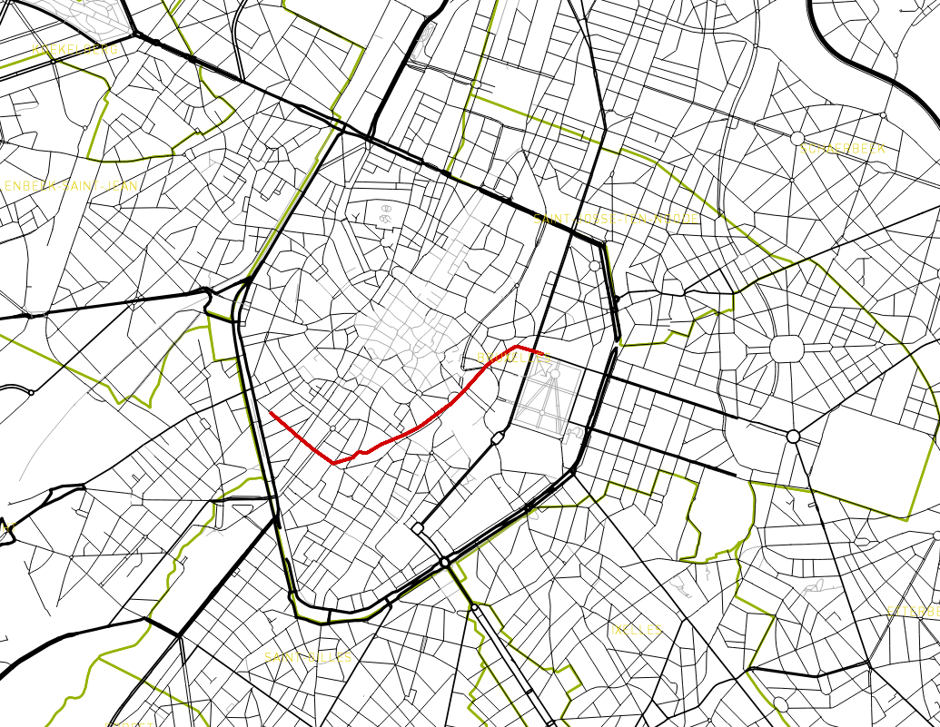
Routing
Get the Longitudinale Profile
An important piece of our developments is to create the longitudinal profile. Here, Excel comes into play with its charting capabilities.
Data are extracted to a CSV file using ogr2ogr.
ogr2ogr -progress -sql "select seq, cost, heading, st_length(geom) length, elevation, slope from test.testrouting"
-f CSV routing.csv PG:"host='<ip>' dbname=routing_slope user='themagiscian' password='*****'"
From there, we plot the data on a graph and we obtain the following one.
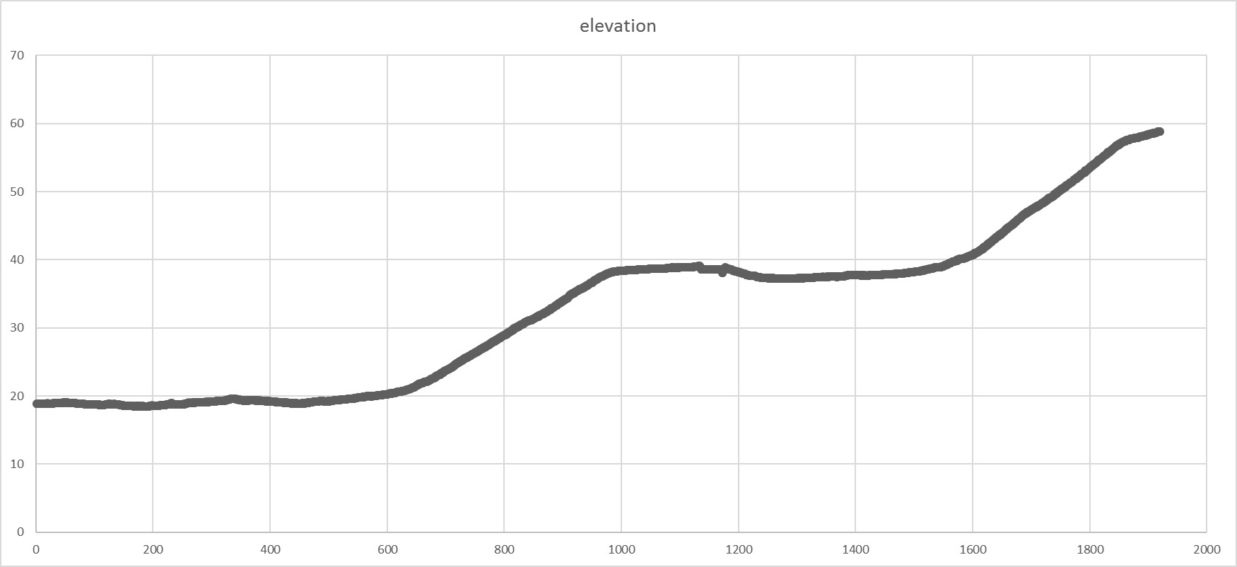
Longitudinal Profile
Conclusions
With free data (AGIV, OSM) and free tools (PostGIS, QGIS, ogr2ogr), we were able to create a routing infrastructure that takes into account the slope in the Best route alternative algorithm. Possible applications could be for elderly people who visit Brussels by bike for them to take the least effort-demand route.
Cheers,
Daniel, themagiscian.com
The Simple and Free PostGIS VS the Complex and Expensive Oracle Spatial
November 21st, 2016Spatial Database battles exists since … the existence of spatial databases! Two most prominent spatial database in the GIS world are Oracle Spatial and PostgreSQL/PostGIS, both having advantages and disadvantages.

While most of the GIS customers are still using file-based data – we are all guilty because we ALL still use Shapefiles – the trends show that more organizations are moving to centralized systems involving spatial databases, more than ever before. Spatial databases offer a lot of advantages file-based system do not have. Here are a few of them (Source). They:
- Handle data more efficiently
- Are better performant
- Are better integrated with external applications
- Take up less space
- Have reduced redundancy risks
- Benefit of the power of SQL with which you can theoretically do anything with the data
- You have more control on the data and processing are less black-boxed
- …
On the other hand, they have a big disadvantage towards file-based systems: they require skills for the implementation, maintenance, usage, etc. (themagiscian.com can help 🙂 ). Small organizations with a few GIS experts, or not trained personal, thus have more difficulties handling bigger systems. It all comes to the need the organization have: Is it just producing maps? Does it need to be interoperable when there’s only one GIS expert in-house? Etc.
In this article, we will compare, from the technical side, PostGIS and Oracle Spatial. We won’t go into installation, configuration, and tuning – we assume we have already up and running systems – but we will only compare the differences in the spatial functions for manipulating geospatial data.
Saying Oracle is more robust than PostGIS begins to be not always true as the overall PostgreSQL community takes the performances very serious. This article shows the advantage of PostGIS over Oracle in both the cold and warm phase when it comes to performance testing. This article is also referenced by this one. Even Oracle itself recognize some best performances done by PostGIS compared to Oracle. Other tests done in March 2016 on very simple queries shows the faster PostGIS.
Let’s be clear: the goal of this article is NOT to advocate for one or the other system in the implementation of a spatial database. It all comes to the purpose of such an implementation, the budget, the goals, etc. We’re just comparing the way the requests are built for doing basic spatial operations.
The exercices are about the handling of data about the municipalities in Belgium for the vectors and a Sentinel-2 scene to illustrate basic tasks for rasters.
Let’s go!
1. Connection as “root”
PostGIS
The command line client is psql
psql -Upostgres -h<ip>
Oracle Spatial
In Oracle, we use sqlplus
sqlplus sys/oracle@<ip>:1521/orcl as sysdba
2. Create User/Schema
PostGIS
Our user “daniel” is created following way
CREATE USER daniel WITH PASSWORD 'daniel';
Oracle Spatial
In Oracle, the concept of user and schema is very different from what it is in PostGIS. We have to see the schema as a user account with all the objects and tables associated with it. We need to add an additional clause to give the basic priviledges to our user
CREATE USER daniel IDENTIFIED BY daniel DEFAULT TABLESPACE daniel_ts;
GRANT CONNECT, RESOURCE TO daniel;
3. Create Spatial Database
PostGIS
In PostGIS, for each database created, we have to enable the spatial extension of the table for all the tables
CREATE DATABASE daniel WITH OWNER daniel;
CREATE EXTENSION postgis;
Oracle Spatial
Nothing to do! What? Yes nothing to do! In the previous step we create a user/schema, which is in fact a set of objects composed of user, objects, tables, views, triggers.
4. Import a Shapefile
PostGIS
For PostGIS, we use the shp2pgsql tool provided with the PostGIS installation. Let’s import our Belgian municipalities shapefile
shp2pgsql -s3812 -d -ggeom -I "[DATAPATH]\Municipalities_A_AdMu.shp" public.a_municipalities
| psql -Udaniel -h<ip> -ddaniel
Oracle Spatial
For Oracle, three methods are at our disposal.
The first being the use of Java classes and the librarie provided by a client instance
java -classpath %ORACLE_HOME%\jdbc\lib\ojdbc7.jar;%ORACLE_HOME%\md\lib\sdoutl.jar;
%ORACLE_HOME%\md\lib\sdoapi.jar oracle.spatial.util.SampleShapefileToJGeomFeature
-h <ip> -p 1521 -s orcl -u daniel -d daniel -t municipalities
-f "[DATAPATH]\Municipalities_A_AdMu.shp" -r 3812 -g geom
The second solution is the use of the ogr2ogr utility
ogr2ogr -progress -lco SRID=3812 -lco GEOMETRY_NAME=geom -nlt MULTIPOLYGON
-nln a_municipalities -f "OCI" -overwrite OCI:daniel/daniel@<ip>/orcl "[DATAPATH]\Municipalities_A_AdMu.shp"
The third solution is using the mapbuilder tool and thus manually uploading the shapefile.
Note that the ogr2ogr for Oracle is much more picky than the shp2pgsql tool for PostGIS. You may have to play with the different import options as every single discrepancy in the shapefile will reject the whole feature during the data loading phase. Be sure the Shapefile is PERFECT!
5. Feature count
PostGIS
This is an easy one
SELECT count(*) FROM a_municipalities;
 count
-------
 589
(1 row)
We have 589 municipalities in Belgium, which is correct.
Oracle Spatial
SELECT count(*) FROM a_municipalities;
 COUNT(*)
----------
 589
6. Get the list of municipalities which are in a radius of 30 km from Brussels, the capital
PostGIS
We use the ST_DWithin function in the WHERE clause
SELECT m2.admunafr FROM a_municipalities m1, a_municipalities m2
WHERE m1.admunafr = 'BRUXELLES' AND ST_DWithin(m1.geom, m2.geom, 30000);
Oracle Spatial
In Oracle Spatial we make use of the SDO_WITHIN_DISTANCE function from the SDO_GEOM package
SELECT m2.admunafr FROM a_municipalities m1, a_municipalities m2
WHERE m1.admunafr = 'BRUXELLES' AND SDO_WITHIN_DISTANCE(m1.geom, m2.geom, 'distance=30000') = 'TRUE' ;
Both results return the same set.
7. Getting the biggest municipality
PostGIS
Usage of the ST_Area function (the units of the result is in km²)
SELECT admunafr, area FROM (
    SELECT admunafr, ST_Area(geom)/1000000 area FROM a_municipalities) t
ORDER BY area desc LIMIT 1;

 admunafr | area
----------+------------------
 TOURNAI | 215.367669469211
(1 row)
Oracle Spatial
Usage of the SDO_AREA function of the SDO_GEOM package. A little bit longer as we have to keep only the first result from the resulting table.
SELECT admunafr, area FROM
     (SELECT admunafr, area FROM
          (SELECT admunafr, SDO_GEOM.SDO_AREA(geom, 0.0005)/1000000 area
          FROM a_municipalities) t ORDER BY area desc) u
 WHERE rownum = 1;

ADMUNAFR AREA
------------------------ ----------
TOURNAI 215,367669
8. Get the 5 municipalities with the most neighbours
PostGIS
We use the function ST_Touches in the WHERE clause and when two municipalities touches, we count 1. The resulting table is then grouped and the ‘1’ summed.
SELECT admunafr, sum(count) neighbours FROM
     (SELECT m1.admukey, m1.admunafr, 1 count FROM a_municipalities m1, a_municipalities m2
     WHERE m1.objectid != m2.objectid AND ST_Touches(m1.geom, m2.geom)) t
GROUP BY admukey, admunafr ORDER BY neighbours DESC LIMIT 5;
 admunafr | neighbours
-----------+------------
 BRUXELLES | 16
 ANVERS | 14
 GAND | 12
 LIEGE | 11
 TONGRES | 11
(5 rows)
No surprise, they are mostly big cities with Brussels having a total of 16 neighbouring municipalities! For your information, here are they
SELECT m2.admunafr FROM a_municipalities m1, a_municipalities m2 WHERE m1.objectid != m2.objectid
AND ST_Touches(m1.geom, m2.geom) AND m1.admunafr = 'BRUXELLES' ORDER BY m2.admunafr;

admunafr
-----------------------
 ANDERLECHT
 ETTERBEEK
 EVERE
 GRIMBERGEN
 IXELLES
 JETTE
 MACHELEN
 MOLENBEEK-SAINT-JEAN
 SAINT-GILLES
 SAINT-JOSSE-TEN-NOODE
 SCHAERBEEK
 UCCLE
 VILVORDE
 WATERMAEL-BOITSFORT
 WEMMEL
 ZAVENTEM
(16 rows)
Oracle Spatial
For Oracle, we use the SDO_RELATE operator with the ‘touch‘ mask
SELECT admunafr, neighbours FROM
     (SELECT admunafr, sum(count) neighbours FROM
          (SELECT m1.admukey, m1.admunafr, 1 count FROM a_municipalities m1, a_municipalities m2
               WHERE m1.objectid != m2.objectid AND SDO_RELATE(m1.geom, m2.geom, 'mask=touch') = 'TRUE') t
     GROUP BY admukey, admunafr ORDER BY neighbours DESC) u
WHERE rownum <=5;

ADMUNAFR NEIGHBOURS
------------------------ ----------
BRUXELLES 16
ANVERS 14
GAND 12
LIEGE 11
TONGRES 11

9. Municipality with longest border (perimeter)
PostGIS
The ST_Perimeter comes into play! (Again, the unit of the result is in km)
SELECT admunafr, perimeter FROM
     (SELECT admunafr, ST_Perimeter(geom)/1000 perimeter FROM a_municipalities) t
ORDER BY perimeter desc LIMIT 1;

 admunafr | perimeter
----------+-----------------
 TOURNAI | 103.241775546157
(1 row)
Tournai, again, has the longest border
Oracle Spatial
The SDO_LENGTH function takes the perimeter here
SELECT admunafr, perimeter FROM (SELECT admunafr, perimeter FROM
     (SELECT admunafr, SDO_GEOM.SDO_LENGTH(geom, 0.0005)/1000 perimeter
     FROM a_municipalities) t ORDER BY perimeter desc) u
WHERE rownum = 1;
ADMUNAFR PERIMETER
------------------------ ----------
TOURNAI 103,241776
10. Most and Least compact municipalities
PostGIS
The compactness of a geometry, in this case the shapes of the municipalities, can have different definitions. In this case, we take the formula corresponding to the area of the municipalitiy DIVIDED by the area of the Circle having the same perimeter. A perfect circle would have a value of 1 and the least compact shape a value near to 0. We thus use here a formula in our query. Notice how we make use of the ST_Perimeter function seen before. From the area of a circle formula, which is R² * pi, and from the perimeter function, which is 2R * pi, we know that the area of an equivalent circle would be Perimeter² / pi.
SELECT admunafr, compactness FROM
     (SELECT admunafr, ST_Area(geom)/(ST_Perimeter(geom)^2 / pi() ) compactness FROM a_municipalities) t
ORDER BY compactness DESC LIMIT 5;

admunafr | compactness
 -------------+-------------------
 MERKSPLAS | 0.171412046968982
 ARENDONK | 0.165099170160105
 LOMMEL | 0.158076966995777
 RIJKEVORSEL | 0.155705115550531
 BRASSCHAAT | 0.154077135253196
 (5 rows)
We see indeed that the shapes of the selected municipalities approaches circles.
SELECT admunafr, compactness FROM (SELECT admunafr, ST_Area(geom)/(ST_Perimeter(geom)^2 / pi() ) compactness
FROM a_municipalities) t ORDER BY compactness ASC LIMIT 5;

admunafr | compactness
 ------------+---------------------
 BAERLE-DUC | 0.00698767111042899
 RAEREN | 0.0269921358361835
 BRUXELLES | 0.0309352964504475
 WAIMES | 0.0364562022393661
 VISE | 0.0364980110812303
 (5 rows)
Notice how these results are coherent. The most compact municipalities are approaching circles while the least compact municipalities are much more stretched, or complicated for the municipality of Baarle-Hertog.
Oracle Spatial
Not much different formulas, but different notation. Notice: there are still no PI value constant in Oracle! We have to hard code the value 3.1415926
SELECT admunafr, compactness FROM (SELECT admunafr, SDO_GEOM.SDO_AREA(geom, 0.005)
     /(POWER(SDO_GEOM.SDO_LENGTH(geom, 0.005), 2) / 3.1415926 ) compactness
     FROM a_municipalities ORDER BY compactness DESC) t WHERE rownum <= 5;
SELECT admunafr, compactness FROM (SELECT admunafr, SDO_GEOM.SDO_AREA(geom, 0.005)
     /(POWER(SDO_GEOM.SDO_LENGTH(geom, 0.005), 2) / 3.1415926 ) compactness
     FROM a_municipalities ORDER BY compactness ASC) t WHERE rownum <= 5;
11. Polygons
PostGIS
We first create the table, then we use the ST_SetGeomFromText function to insert our point. Notice: We construct a triangle where the points are the city centers of Antwerp, Brussels and Namur.
DROP TABLE f_polygons;
CREATE TABLE f_polygons (
     id serial PRIMARY KEY,
     description varchar(32),
     geom GEOMETRY(POLYGON, 3812)
);

INSERT INTO f_polygons(description, geom) VALUES ('First Polygon',
     ST_Transform(
          ST_SetSRID(
               ST_GeometryFromText(
                    'POLYGON((4.4033 51.21972, 4.348611 50.85028, 4.867222 50.46667, 4.4033 51.21972))'),
                         4326), 3812));
We have the coordinates in 4326 lon, lat but we need them in 3812 (Belgian Lambert 2008). ST_Transform is use for doing the reprojection. The way the geometry is described is the WKT format, an OGC standard. The last point has to be repeated to close the boundary linestring.
Oracle Spatial
DROP TABLE f_polygons;
CREATE TABLE f_polygons (
 id NUMBER GENERATED BY DEFAULT ON NULL AS IDENTITY,
 description varchar(32),
 geom SDO_GEOMETRY
 );

ALTER TABLE f_polygons ADD (
 CONSTRAINT polygons_pk PRIMARY KEY (id)
 );

INSERT INTO f_polygons(description, geom) VALUES ('First Polygon', SDO_CS.TRANSFORM(
MDSYS.SDO_GEOMETRY(
2003,
4326,
NULL,
MDSYS.SDO_ELEM_INFO_ARRAY(1,1003,1),
MDSYS.SDO_ORDINATE_ARRAY(4.4033, 51.21972, 4.348611, 50.85028, 4.867222, 50.46667, 4.4033, 51.21972)
), 3812));

DELETE FROM USER_SDO_GEOM_METADATA WHERE TABLE_NAME = 'F_POLYGONS';
INSERT INTO USER_SDO_GEOM_METADATA (TABLE_NAME, COLUMN_NAME, DIMINFO, SRID)
VALUES (
 'F_POLYGONS',
 'GEOM',
 SDO_DIM_ARRAY (
 SDO_DIM_ELEMENT('Long', -180, 180, 0.5),
 SDO_DIM_ELEMENT('Lat', -90, 90, 0.5)),
 3812);

DROP INDEX f_polygons_idx;
CREATE INDEX f_polygons_idx ON f_polygons (geom) INDEXTYPE IS MDSYS.SPATIAL_INDEX;
What the hell! All of this for creating a polygon with three points? YES! Welcome to Oracle!
No OGC, nothing clear text (see the numbers everywhere, they are keys to specify geom types…) and thus no OGC standard, and the spatial index is mandatory otherwise no spatial operation is possible. Notice also the mandatory insert into the USER_SDO_GEOM_METADATA table … A lot of things to take into account here!
For the geometry, we use the MDSYS.SDO_GEOMETRY operator with
- 2003 being for a two dimensional polygon (yes yes!)
- 4326 the srid
- NULL? Yes! In case you would like your polygon to be a point (huh?)
- SDO_ELEM_INFO_ARRAY(1,1003,1) : where the parameters are respectively for the starting offet (see the next parameter), defining an exterior polygon ring and telling the system to connect point with straight lines. OKAY!
- And finally MDSYS.SDO_ORDINATE_ARRAY with all the coordinates we need! Important: It seems that finally they drop their constraint to specify the coordinates counterclockwise! Counterclockwise and clockwise now both work! Waow!
12. Points
PostGIS
Let’s see how it is to create points …
DROP TABLE g_points;
CREATE TABLE g_points (
     id serial PRIMARY KEY,
     description varchar(32),
     geom GEOMETRY(POINT, 3812)
);
INSERT INTO g_points(description, geom) VALUES ('First Point', ST_Transform(
     ST_SetSRID(
          ST_Point(4.348611, 50.85028), 4326), 3812));
The same workflow as for the polygons except that we use the ST_Point constructor.
Oracle Spatial
DROP TABLE g_points;
CREATE TABLE g_points (
     id NUMBER GENERATED BY DEFAULT ON NULL AS IDENTITY,
     description varchar(32),
     geom SDO_GEOMETRY
 );

ALTER TABLE g_points ADD (
     CONSTRAINT g_points_pk PRIMARY KEY (id)
);

INSERT INTO g_points(description, geom) VALUES ('First Point',
     SDO_CS.TRANSFORM(
     MDSYS.SDO_GEOMETRY(
          2001,
          4326,
          MDSYS.SDO_POINT_TYPE(4.348611, 50.85028, NULL),
          NULL,
          NULL
 )
 , 3812
 ));

DELETE FROM USER_SDO_GEOM_METADATA WHERE TABLE_NAME = 'G_POINTS';
INSERT INTO USER_SDO_GEOM_METADATA (TABLE_NAME, COLUMN_NAME, DIMINFO, SRID)
VALUES (
 'G_POINTS',
 'GEOM',
 SDO_DIM_ARRAY (
 SDO_DIM_ELEMENT('Long', -180, 180, 0.5),
 SDO_DIM_ELEMENT('Lat', -90, 90, 0.5)),
 3812);

DROP INDEX g_points_idx;
CREATE INDEX g_points_idx ON g_points (geom) INDEXTYPE IS MDSYS.SPATIAL_INDEX;
Wow again! But here we use other codes in the SDO_GEOMETRY constructor. The third parameter, which was NULL for the polygons, is now filled with values for specifying a point. It is more performant to separate point and polygon creation they say.
13. Raster Import
PostGIS
Let’s see how both spatial databases handle the import of rasters. We’re using Sentinel-2 cloud-free scenes of the Belgian coast taken the 31st of October 2016.
raster2pgsql -c -C -s 32631 -f rast -F -I -M -t 100×100 [PATHTODATA]/B02.jp2 public.h_b02 | psql -Udaniel -h<ip> -ddaniel
raster2pgsql -c -C -s 32631 -f rast -F -I -M -t 100×100 [PATHTODATA]/B03.jp2 public.h_b03 | psql -Udaniel -h<ip> -ddaniel
raster2pgsql -c -C -s 32631 -f rast -F -I -M -t 100×100 [PATHTODATA]/B04.jp2 public.h_b04 | psql -Udaniel -h<ip> -ddaniel
raster2pgsql is a utility coming with the PostGIS extension. The following parameters stand for.
- -c: create the table
- -C: apply raster constraints
- -s: specify the ouput srid
- -f: specify the name of the raster column
- -F: adds a column with the name of the file
- -I: Creates the index
- -M: Vacuum raster table
- -t: specifies, in pixels, the size of the tiles in which the raster has to be cut
Oracle Spatial
In Oracle Spatial, we first need to create the welcoming raster tables! Nothing created by a potential import script!
After the creation of the tables, we need to create the raster data tables: the rdt. The first containing the raster, the other the data associated with them.
DROP TABLE h_belgium;
CREATE TABLE h_belgium(
     georid number primary key,
     source_file varchar2(80),
     description varchar2(256),
     georaster sdo_georaster,
     load_duration number,
     pyramid_duration number
);

DROP TABLE h_belgium_rdt;
CREATE TABLE h_belgium_rdt OF sdo_raster (
     PRIMARY KEY (
         rasterId, pyramidLevel, bandBlockNumber,
         rowBlockNumber, columnBlockNumber)
)
LOB (rasterblock) STORE AS SECUREFILE (NOCACHE NOLOGGING);

-- INSERT INTO USER_SDO_GEOM_METADATA
DELETE FROM user_sdo_geom_metadata WHERE table_name in ('H_BELGIUM');
INSERT INTO user_sdo_geom_metadata (
     table_name, column_name, diminfo, srid
)
VALUES (
     'H_BELGIUM',
     'GEORASTER.SPATIALEXTENT',
     sdo_dim_array(
     sdo_dim_element('LONG', 499980, 508980, 0.05),
     sdo_dim_element('LAT', 5699000, 5700000, 0.05)
     ),
 32631
);
COMMIT;

EXECUTE sdo_geor_admin.registerGeoRasterColumns;
SELECT * FROM THE (SELECT SDO_GEOR_ADMIN.listGeoRasterColumns FROM DUAL);
EXECUTE sdo_geor_admin.registerGeoRasterObjects;
Then, we can use … GDAL! You could use the GeoRasterLoader class provided with the Georaster Tools but … good luck!
gdal_translate -of georaster [PATHTODATA]\B02.jp2" georaster:daniel/daniel@<ip>:1521/orcl,H_BELGIUM,georaster
-co blockxsize=512 -co blockysize=512 -co blockbsize=3 -co interleave=bip -co srid=32631 -co
"insert=values(1, '31UES20161031/b02.jp2', 'H_BELGIUM S2 B02', sdo_geor.init('H_BELGIUM_RDT', 1),null,null)" -co compress=deflate
gdal_translate -of georaster [PATHTODATA]\B03.jp2" georaster:daniel/daniel@<ip>:1521/orcl,H_BELGIUM,georaster
-co blockxsize=512 -co blockysize=512 -co blockbsize=3 -co interleave=bip -co srid=32631 -co
"insert=values(2, '31UES20161031/b03.jp2', 'H_BELGIUM S2 B03', sdo_geor.init('H_BELGIUM_RDT', 2),null,null)" -co compress=deflate
gdal_translate -of georaster [PATHTODATA]\B04.jp2" georaster:daniel/daniel@<ip>:1521/orcl,H_BELGIUM,georaster
-co blockxsize=512 -co blockysize=512 -co blockbsize=3 -co interleave=bip -co srid=32631 -co
"insert=values(3, '31UES20161031/b04.jp2', 'H_BELGIUM S2 B04', sdo_geor.init('H_BELGIUM_RDT', 3),null,null)" -co compress=deflate
See how we have to initialize the rasters.
After the import, we must create the index to make the georaster fully exploitable.
-- CREATE INDEX
DROP INDEX H_BELGIUM_SX;
CREATE INDEX H_BELGIUM_SX
 ON H_BELGIUM (georaster.spatialextent)
 indextype IS mdsys.spatial_index;
COMMIT;
With a nice True Colour band combination, we got the following result. Example with the city of Bruges near the Belgian coast.
Conclusion
Both PostGIS and Oracle Spatial have advantages and disadvantages. PostGIS seems however easier to install, to manage and to manipulate. It is futhermore totally FREE and at the hand of every small to big business. Oracle Spatial still has a big and good reputation with a hard-working team behind the product and a proven record of robustness.
Cheers,
Daniel
The 2012 Presidential Election Map using PostGIS, Geoserver and OL3
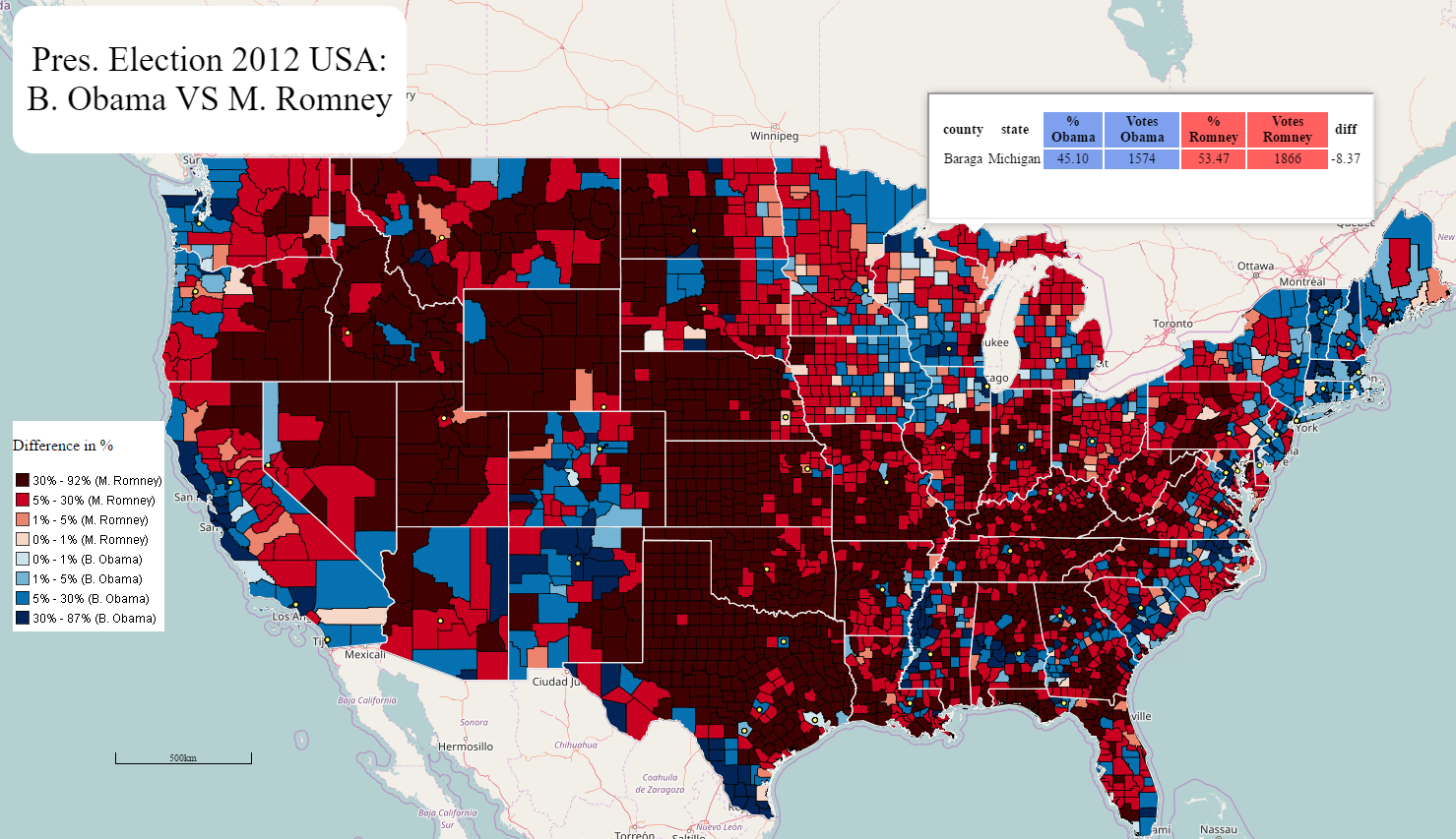
November 12th, 2016The news of the beginning of the week was monopolized by the US presidential election. During the last few months, a lot of interactive maps flourished on the internet showing the tendencies in the polls. This gave me the idea to make my own interactive maps!
It seems the data per county for the 2016 election are not yet freely available. So I did an election map of the … 2012 presidential election. This article is about the creation of such a map using OpenSource tools: QGIS, PostGIS, Geoserver and OpenStreetMap.
Note: This web application is not online as I do not have the infrastructure to host it.
The symbology represents the different in percentage between the vote going to Barack Obama VS Mitt Romney. The light colour counties show where there is an almost tie. The redder the county, the more vote for the Republican Nominee vs the Democrate, and vice-versa with blue.
Get the data
The first step is to get the data. The dataset I found comes from the Guardian website.
The Excel file is rather raw and needs to be cleaned up.
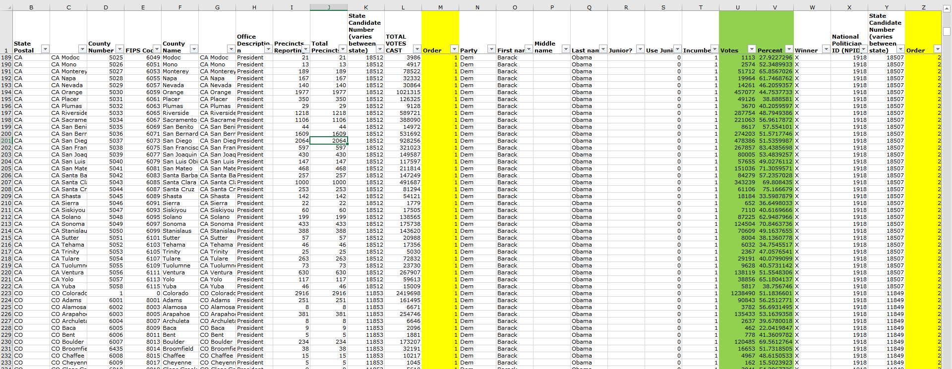
There are two sheets in this Excel file. The first shows the direct confrontation between Barack Obama and Mitt Romney. Strangely, some states, such as Colorado, are not covered. The second sheet of the document contains all the US counties and the votes for every candidate, even for Colorado. That means, third party candidates are also listed but we want to focus only of the two major actors of this election: Barack Obama and Mitt Romney. The Excel sheet has thus to be cleaned!
Clean the data
The way I approached this problem is the following: I only need information about the county, the total votes and the percentage for Barack Obama and for Mitt Romney. A concatenate formula helps me with creating INSERT scripts. Here’s one of the 4639 scripts:
INSERT INTO results(state_postal, county_name, fips, obama_vote, obama_percent, romney_vote, romney_percent, total_votes) VALUES ('CA', 'San Bernardino', 6071, 274203, 51.5717746364437, 245468, 46.1673299579456, 531692);
Data Loading and preparation
As of always, we’re using an underlying PostGIS database to store and manage the data.
Our database is called usa2012election we’re loading first three geographic layers: one for the counties, one for US States and one for the biggest cities. All of them are freely available on the ArcGIS platform. The data loading is performed using the shp2pgsql tool.
shp2pgsql -s4326 -c -ggeom -I "[...]\COUNTIES.shp" public.counties | psql -U<user> -h<ip>-dusa2012election
shp2pgsql -s4326 -c -ggeom -I "[...]\cb_2015_us_state_500k.shp" public.states | psql -U<user> -h<ip>-dusa2012election
shp2pgsql -s4326 -c -ggeom -I "[...]\USCITIES.shp" public.cities | psql -U<user -h<ip> -dusa2012election
A lot of information is unnecessary in the county table. We clean all the fields we are not interested in.
ALTER TABLE counties DROP COLUMN pop_sqmi , DROP COLUMN pop2010 , DROP COLUMN pop10_sqmi , [...];
ALTER TABLE cities DROP COLUMN gid, DROP COLUMN class, DROP COLUMN st, DROP COLUMN stfips, [...];
DELETE FROM cities WHERE population < 100000 AND capital IS NULL;
The table containing the data from the Excel sheet is created here. We call it “results”;
DROP TABLE results;
 CREATE TABLE results (
 id serial PRIMARY KEY,
 state_postal varchar(2),
 county_name varchar(20),
 fips numeric(5),
 obama_vote float,
 obama_percent float,
 romney_vote float,
 romney_percent float,
 vote_balance float,
 total_votes numeric(7)
 );
We can now execute the whole bunch of insert scripts we created in the Excel file.
INSERT INTO results (state_postal, county_name, fips, obama_vote, obama_percent, romney_vote, romney_percent, total_votes) VALUES (‘WV’, ‘Wood’, 54107, 11067, 32.9375, 21980, 65.4166666666667, 33600);
INSERT INTO results (state_postal, county_name, fips, obama_vote, obama_percent, romney_vote, romney_percent, total_votes) VALUES (‘WV’, ‘Wyoming’, 54109, 1575, 21.0112059765208, 5751, 76.7209178228389, 7496);
INSERT INTO results (state_postal, county_name, fips, obama_vote, obama_percent, romney_vote, romney_percent, total_votes) VALUES (‘WY’, ‘Wyoming’, 0, 68780, 27.9838069857803, 170265, 69.2739589478609, 245785);
INSERT INTO results (state_postal, county_name, fips, obama_vote, obama_percent, romney_vote, romney_percent, total_votes) VALUES (‘WY’, ‘Albany’, 56001, 7445, 46.3805133316721, 7851, 48.9097931721904, 16052);
[…]
The FIPS, the field that identifies uniquely every county, is not of the same data type in the tables results and county. It must be as we’ll do a join between both tables! The FIPS in the results table is converted from integer to varchar.
ALTER TABLE results ALTER COLUMN fips TYPE varchar(5) USING cast(fips AS varchar(5));
The FIPS in the geometric table are of type varchar and contains a leading zero. We have to make sure they don’t so they can be joined with the results table. Only the States in the beginning of the alphabet have a leading zero as FIPS..
UPDATE counties SET fips = LTRIM(fips, '0') WHERE
state_name = 'Alaska' OR state_name = 'Alabama' OR
state_name = 'Arkansas' OR state_name = 'Arizona' OR
state_name = 'California' OR state_name = 'Colorado' OR
state_name = 'Connecticut' OR state_name = 'District of Columbia' OR
state_name = 'Delaware';
We perform, finally, our join between both tables. We store the result in a view we will later use in Geoserver.
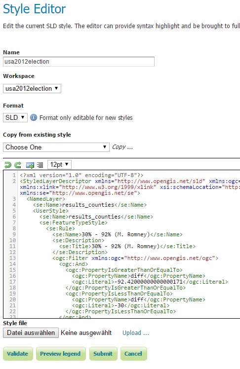
DROP VIEW results_counties;
 CREATE VIEW results_counties AS SELECT c.name County, c.state_name State,
round(cast(r.obama_percent as numeric), 2) "% Obama",
round(cast(r.obama_vote as numeric)) "Votes Obama",
round(cast(r.romney_percent as numeric), 2) "% Romney",
round(cast(r.romney_vote as numeric)) "Votes Romney",
round(cast(r.vote_balance as numeric), 2) "% diff",
c.geom FROM counties c JOIN results r ON c.fips = r.fips;
Notice how we round the values so the reading will be more comfortable in the web app.
Configure Geoserver
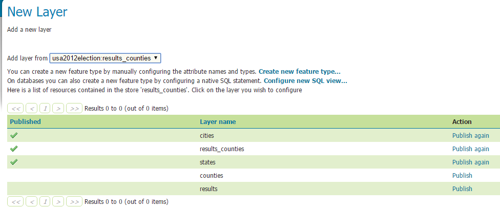
The idea is to server the data via Geoserver. Here are the steps
- Create a workspace, we call it usa2012election
- Create a store
- Add our two layers (states and cities) and our view (results_counties)
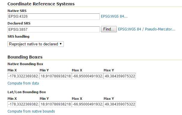
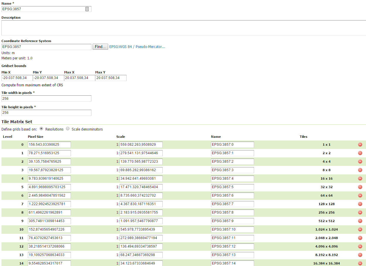
For the configuration of the layer, pay attention to the SRS! Our original data is in 4326, and we need 3857 as it is the default one used in OpenLayers 3! The other reason is that we will use an OpenStreetMap Background as thus only 3857 is accepted.
The styles are in SLD format and were created in QGIS. The three SLD files, one for each layer and the view, are appended.
Last but not least, we need our application to be performant (of course)! The step here is to defined Tile Caches. This is mandatory in our case as the County layer is quite heavy and takes somes seconds to load. This is not good.
Create first an EPSG 3857 Gridset
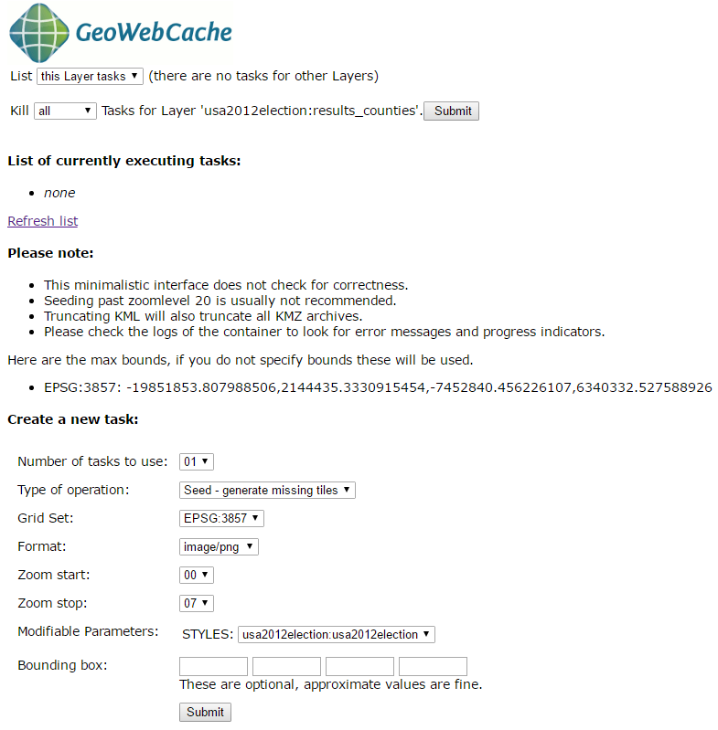
Then, generate the tiles for each of the layers.
OpenLayers 3 Client Development
The final part is configuring the Web client using OpenLayers 3.
The first step is quite basic we the definition of our html file. Three parts here: the map, the title bar and the legend.
<!DOCTYPE html>
 <html>
 <head>
 <title>USA 2012 ELECTION</title>
 <meta charset="utf-8">
 <link href="css/ol.css" rel="stylesheet">
 <link href="css/usa2012election.css" rel="stylesheet">
 </head>
 <body>
 <div id="title">
 <p>Pres. Election 2012 USA: B. Obama VS M. Romney</p>
 </div>
 <div id="legend">
 <p>Legend</p>
 <img src="[...]/geoserver/usa2012election/ows?service=WMS&request=GetLegendGraphic&format=image%2Fpng&width=20&height=20&layer=results_counties&style=usa2012election">
 </div>
 <div id="map"></div>
 <div id="popup" class="ol-popup">
 <a href="#" id="popup-closer" class="ol-popup-closer"></a>
 <div id="popup-content"></div>
 </div>
 <script src="js/ol.js"></script>
 <script src="js/OpenLayers.js"></script>
 <script src="js/draw.js"></script>
 </body>
 </html>
Our three layers are added via this way.
var params = {
 LAYERS: 'usa2012election:cities',
 TRANSPARENT: 'false',
 FORMAT: 'image/png'
 };
cities = new ol.layer.Tile({
 source: new ol.source.TileWMS({
 url: '[...]/geoserver/gwc/service/wms?SRS=EPSG:3857',
 params: params
 })});
var params = {
 LAYERS: 'usa2012election:states',
 TRANSPARENT: 'false',
 FORMAT: 'image/png'
 };
states = new ol.layer.Tile({
 source: new ol.source.TileWMS({
 url: '[...]/geoserver/gwc/service/wms?SRS=EPSG:3857',
 params: params
 })});
 var params = {
 LAYERS: 'usa2012election:results_counties',
 TRANSPARENT: 'false',
 FORMAT: 'image/png'
 };
 result = new ol.layer.Tile({
 source: new ol.source.TileWMS({
 url: '[...]/geoserver/gwc/service/wms?SRS=EPSG:3857',
 params: params
 })});
Notice how we get the most of performances using the gwc application. It uses the caches we generated in Geoserver.
Finally, we add a phantom underlying layer which is only used for the GetFeatureInfo functionnality. It is called each time we click on the map to get the relevant information about how many people voted for who.
 var wmsSource = new ol.source.TileWMS({
 url: 'http://localhost:8080/geoserver/usa2012election/wms',
 params: {
 'LAYERS': 'usa2012election:results_counties'},});

var wmsLayer = new ol.layer.Tile({
 source: wmsSource});

map.on('singleclick', function(evt) {
 document.getElementById('popup').innerHTML = '';
 var viewResolution = (view.getResolution());
 var coordinate = evt.coordinate;
 var url = wmsSource.getGetFeatureInfoUrl(
 coordinate, viewResolution, 'EPSG:3857', {
 'INFO_FORMAT': 'text/html'
 });
 if (url) {
 document.getElementById('popup').innerHTML =
'<iframe width="450px" height="125px" border-width="0px"
border-radius:"200px" seamless src="' + url + '"></iframe>';
}
 overlay.setPosition(coordinate);});
Finally, add the layers to the map.
 map.addLayer(result);
 map.addLayer(states);
 map.addLayer(cities);
One last thing! The GetFeatureInfo returns pieces of information that are not necessary to the user. These are the fid and the id. For resolving this issue, we define a file called content.ftl in the Geoserver data folder. We will format the returning information to send to the user.
<table class="featureInfo">
 <caption class="featureInfo"></caption>
 <tr>
<#list type.attributes as attribute>
 <#if !attribute.isGeometry && attribute.name != "id">
 <th >${attribute.name}</th>
 </#if>
</#list>
 </tr>

<#assign odd = false>
<#list features as feature>
 <#if odd>
 <tr class="odd">
 <#else>
 <tr>
 </#if>
 <#assign odd = !odd>

<#list feature.attributes as attribute>
 <#if !attribute.isGeometry && attribute.name != "id">
 <td>${attribute.value}</td>
 </#if>
 </#list>
 </tr>
</#list>
</table>
<br/>
At last, wrap the all application in a very nice css and you got the result we observe in the short introductory video!
All the scripts are available here to reproduce at home!
I am now waiting the 2016 Presidential Election Results by Counties to make and publish an updated map!
Enjoy for recreating your own presidential election map!
Cheers,
Daniel
Is upwork.com actually working for GIS professionals?
October 15th, 2016The story
I created an account as a freelancer on the upwork.com website a year ago, hoping I could make some extra money while doing GIS as a hobby. Since then, after having spend hours to apply to hundreds of proposals, I could only manage to get … 1 mission.
For information, upwork.com is a website where independent professionnals meet. The ones having challenges to be solved and the others having the skills. The numbers are telling: 12 million registered freelancers, 5 million registrered clients, 3 million jobs posted annually, $1 billion as a total.
Not too bad! But a general question that comes to me about all my failures: When I apply, am I doing something wrong?
When I apply to a job proposal, I make sure to provide the customer with at least a small prototyp of what is asked. An example? A French customer asked to digitize as precise as possible a set of 20 buildings spotted on a pdf document. The documents to provide to the customer were the data digitized in shapefile and in KML. This was just the “test” as the whole mission was about a thousand of buildings. They asked all the applicants to show their skills and they would grant the best proposal. So I did digitize their 20 buildings that took me one hour. The input document was bad: No spatial reference was given so I had to search for their buildings first. What about the resolution of the final document? What about the bad “map” on the pdf (it stretches in all directions)?
Guess what ? No answer.
Another example that comes up to my mind is a scientist who studies birds’ journeys. The birds are equipped with a GPS and data are collected. The question was, how to get these data into KML and making it possible to make an animation in Google Earth. So I grabbed his sample file, converted it into KML and made it possible to play with the timeline. It also took me an hour as I had to choose the right KML tags and knowing how the X, Y, Z, and time are formatted. Notepad++ was my best friend. So I sent him the sample in KML format but for one bird. Note: later on, I published a similar article about this.
Guess what ? No answer.
A bigger mission was about the set up of an infrascture involving geoserver, PostGIS and Openlayers on top of that. As I already did some work about it in this blog, I feel at ease in the mission proposed. So I joined to my cover letter a lot of example, screenshots and even a small video showing what I was capable of. It also took me some time to prepare all of this…
Guess what ? No answer.
Ohhw! I got a successful story to tell anyway! … but I had to decline! A freelancer on Upwork contacted me as he was interested for me to write articles for his website. Its bid was a 100$. I said, well, this is not so much for an article as I personnally take from 20 to 30h per technical article! Writing a technical article for themagiscian.com This includes getting the data, processing, wrapping the result, do it again when I am not satisfied by the results or if I learn doing better, and finally write the article. He said “Could you write 2 articles for me for that price?”. And this was the end of the story.
The only succesful mission I got was more a confidence relationship than truly a “tender” where freelancers are applying and bidding. I worked 14h for a swiss customer doing calculations and maps about energy consumptions (fuel, solar, geothermy, etc.) – VERY CHALLENGING and I enjoyed the fun!
Analyses of my failures
I got 6 years of experience in the GIS field and I am in my 11th year doing GIS, master degree included. I worked for big companies (Erdas, Hexagon, Esri, and for two growing startups: Oscars and Quadratic). Beside that, I hold the blog themagiscian.com I created two years ago. I am at ease with GIS technologies and I guess I have a broad vision of spatial software architecture.
So what is going wrong?
First, as looking at the profiles of the other GIS freelancers, one could see that there is a lot of competition. A very BIG competition and you have to stand out of the crowds when applying. I attach to my applications a targeted cover letter with screenshots, gif animations, sample results, and sometimes videos. But this is apparently not enough. Are these other freelancers who got the missions doing the same? How are THEY standing out of the crowds?
Second, the rates of the freelancers! My rate is at $38.75 per hour, which is far above the average rates asked by most of the other GIS freenlancers. This is my very lowest bound as I consider myself as an expert, and I try to apply to the job proposals that ask for skilled experts.
Third, I guess people on Upwork are focused only on the final price. I am well above average with my rates and this is not in my favour. I once saw a Nowergian customer stating clearly in the bottom of his proposal: “We’re searching for someone from India preferably.” This is understandable in the way that, if you are looking for a professional for long-term professional relations, you probably wouldn’t search for an expert on Upwork but you would seek for a service provider in your geographic area, and meet him in person.
Back to the initial question: Is upwork.com actually working for GIS professionals?
My experience on Upwork
After a year on this freelancer exchange platform, I have to say that I am not convinced at all. I spent a lot of time trying to get a mission and I think I am more wasting my time than anything else. I keep however optimistic in the way I am keeping my account and sometimes apply to challenging missions!
Who knows? Maybe one day fishes will bite!
Cheers,
Daniel
Evolution of an area using Sentinel-2 and Time Series
October 9th, 2016The European Commission’s Copernicus programme makes it possible to have a snapshot of Earth every 5 days in the multispectral bands. I already covered several applications of Sentinel-2 imageries:
- Full Sentinel-2 cloud-free mosaic of Belgium!
- Agriculture and Sentinel-2: an unsupervised temporal classification
- Change detection using Sentinel-2 and PostGIS
- Earthquake in Amatrice, Italy: Before/After with Sentinel-2
A zillion of information can be gathered out of every single scene. It does not, however, tell us where these things we’re seeing are coming from, and where they are going to. To do this, we need several scenes of the same area but taken at different moment. Or, in other word, we need to use time series to follow the evolution of an area.
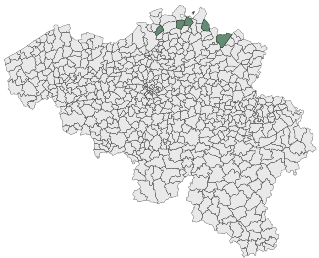
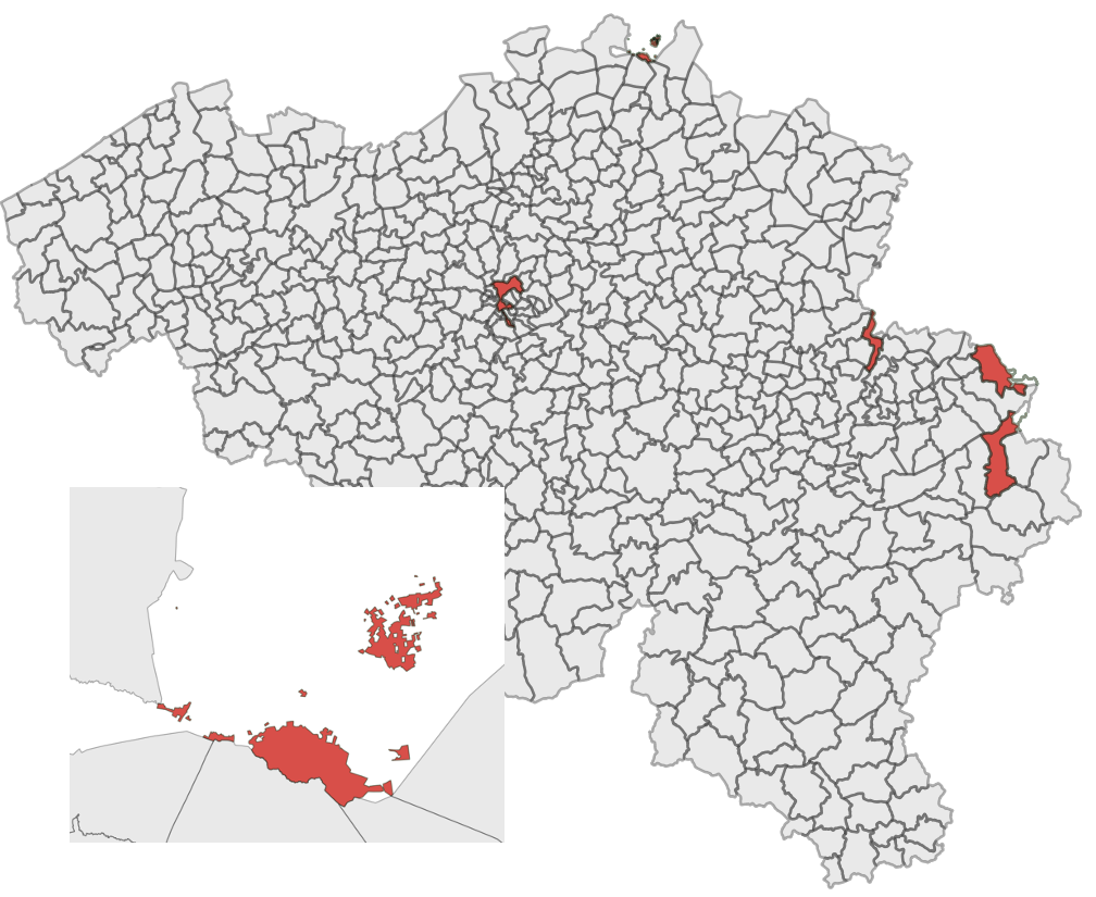
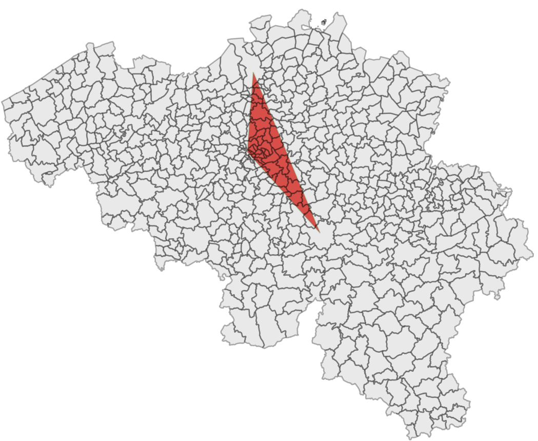
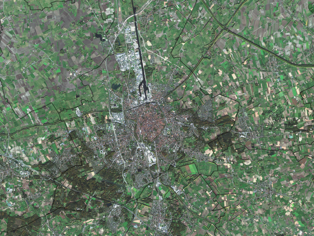
Our study area is the Northen part of Liege in Belgium. We’ve taken several Sentinel-2 scenes between the period going from the 1st of May 2016 and the 25th of September 2016. The evolution of the agricultural fields provides a lot of information, going from the first moments of growth, to maturity and harvest. Notice the data were collected using the method already described here.
The first animated gif file is in true color. This series of scenes is very valuable when used with an agricultural calendar. One could guess of which crop type the fields are knowing the time of harvest period.
As summer peak approaches, we see the overall vegetation become greener. The first harvest wave occurs in the month of June. The first bare lands are most probably hay fields. July sees the biggest harvest season with wheat, sugar beets, peas, etc. Corn is harvested during the September month and the last green fields can be of maize. For the full explanations, please see following article: http://www.quadratic.be/en/le-suivi-de-levolution-des-cultures-en-utilisant-les-imageries-satellitaires/ .
Another intersting time series is about the band combination 5, 4 and 3. It corresponds to the NIR-R-G band combination. This indicator is often used to characterize plants’ health.
Bright red corresponds to healthy vegetation while the more pinkish areas shows some less active plants. Bare land appears clear blue and water very dark as it absorbs almost every wavelength.
The last example of times series that can give additional information is showing the evolution of the Normalized Difference Vegetation Index (NDVI). This index characterizes the photosynthetical activity. The greener the field hereunder, the more active it is. This index is not to be confused with the biomass productivity of a field.
The Time Series is very intersting way to analyse what happens on Earth. The frequent revisit of the Sentinel-2 satellite makes it possible, in theory, to add a new scene to the time series every 5 days. Our example is about agriculture and can be applied to a vast majority of domains! The best example was our change detection articles:
- Change detection using Sentinel-2 and PostGIS
- Earthquake in Amatrice, Italy: Before/After with Sentinel-2
If you’re more interested in Sentinel-2 and agriculture, do no hesitate to follow the company Quadratic.
Cheers,
Daniel
Full Sentinel-2 cloud-free mosaic of Belgium!
October 2nd, 2016The Copernicus’s Sentinel-2 programme makes it possible to have a full mosaic coverage of any point in Europe with a revisit of 5 days at the Equator, provided no clouds come to ruin the party. The resolution of 10 m for the visible bands 2, 3 and 4 are also very interesting making it possible to spot quite reasonable details.
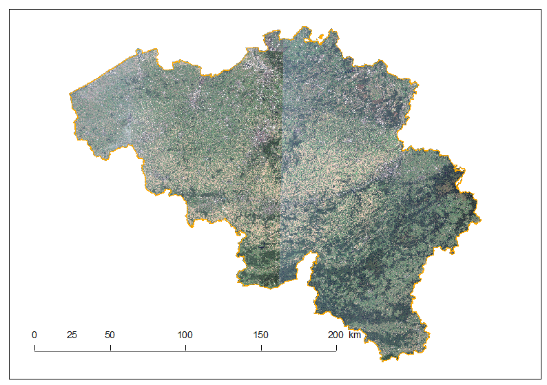
In this article, I created a mosaic with the most recent individual cloud-free Sentinel-2 granules covering Belgium. That means, the timestamp is different depending on the region you look. For the full workflow I’ve done creating this mosaic, please see here at the bottom of the article.
The full cloud-free Sentinel-2 mosaic of Belgium is of course free, please just ask and I will give you and I will provide it to you 🙂
As you notice, each of the granule were not properly color-balanced. It seems our Belgium is divide in two as a seam is clearly visible. Unfortunately, I did not find any way for a perfect color-balance in this area.
Let us discover Belgium using this mosaic.
Our first stop is in the East of Belgium, with the Spa-Francorchamps Formula-1 track every fan knows about. Also known as the most beautiful circuit in the world, the track is 7 km long – the longest of the F1 season – and is located in the village of Francorchamps (which is part of the municipality of Stavelot and not Spa despite its name). We recognize, in the middle, the paddocks and the curve of La Source, just before the Eau rouge. The curve of Les Combes and Stavelot are respectively in the South East and West. If you past by, do not miss a walk in the beautiful surrounding Ardennes Region.
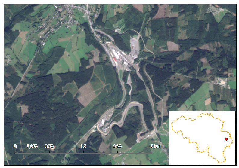
The second stop is Brussels-Airport, the center of March 2016 terrorist attacks. Depiste being called “Brussels-Airport”, tarmac and infrastructures are all located in the Flemish Region, just in the North-East of the Brussels Region. The three runways are clearly visible as well as all the surrounding houses. Urbanisation is very dense near the airport, which causes a lot of political frictions in the country.
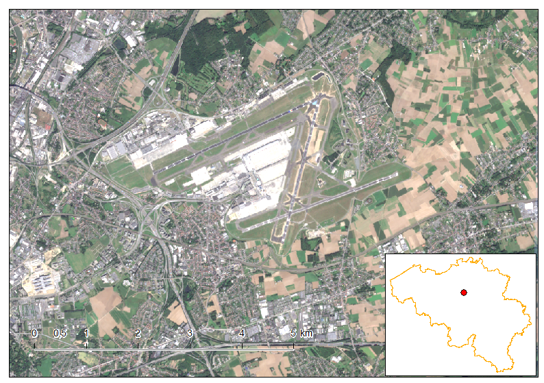
Our next stop is in the Hoge Kempen National park, the only one national park in Flanders. Covereing a total of 60 km², A lot of extraction activities did occur in this region and now it has become a tourist attraction for the beauty of the nature recovery. The waterbody in the South centre seems purple, unlike all the other waterbodies. Taking pictures from space is not like taking a picture on Earth. The atmosphere layer to cross is much more thicker and the wavelengths most altered are in the blue area. It is hence difficult to recover perfectly the colors, so here is the case as well.
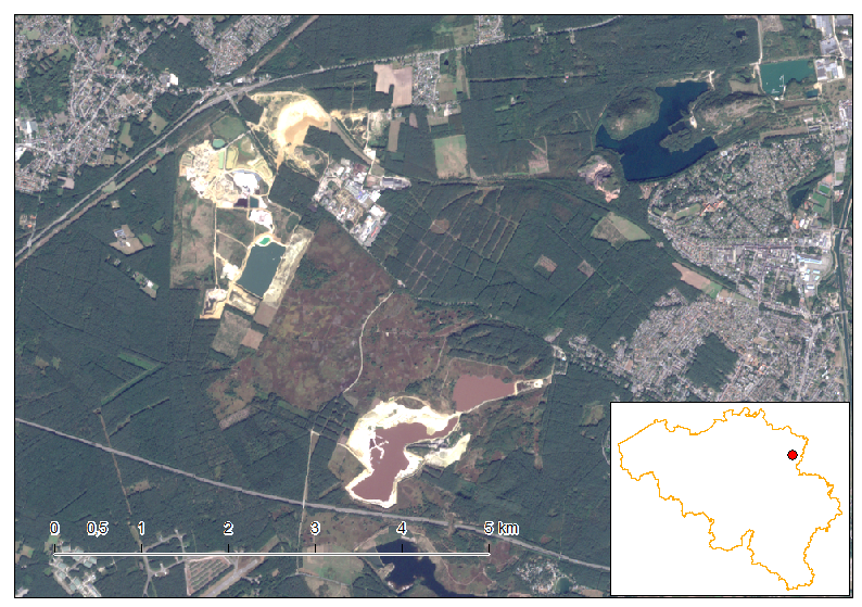
The King’s residence palace in Laeken, just 5 km from the Brussels’s city center. A beautiful park as big as 6 km² has numerous waterbodies, tennis courts and, most importantly, hosts the “Serres Royales”. It is an important collection of plants and flowers and is open to the public only during 3 weeks per year. Really worth it when you are in the area during the Easter period!
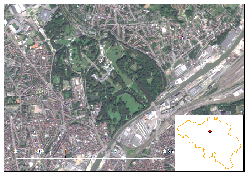
The city of Antwerp hosts the biggest maritime port of the country, and the third biggest maritime port in Europe after Rotterdam (NL) and Hamburg (DE). The cities lies at the mouth of the River Scheldt Worth telling is that the city is ranked number one in diamond trade. 80% of all the diamonds in the world transits through Antwerp. An important tourist attraction is the Antwerp zoo, founded in 1843, and is the oldest zoo on Earth.
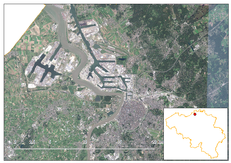
This fragmented area is no other than the municipality of Baarle-Hertog. The overall Belgian exclave has “holes” which are part of The Netherlands. This administrative anomaly comes for the period where borders have been drawn between the freshly born Belgium and The Netherlands. Representative were quite in accord with the separation line between both countries except in this area particular area. A lot of Belgian and Dutch owner were living there next to another. Archives have to be retrieved and documents dating up to the 1100’s were used to defined the border. Now beeing a tourist place where you can sit on a terrace in Belgium while ordering in the Netherlands.
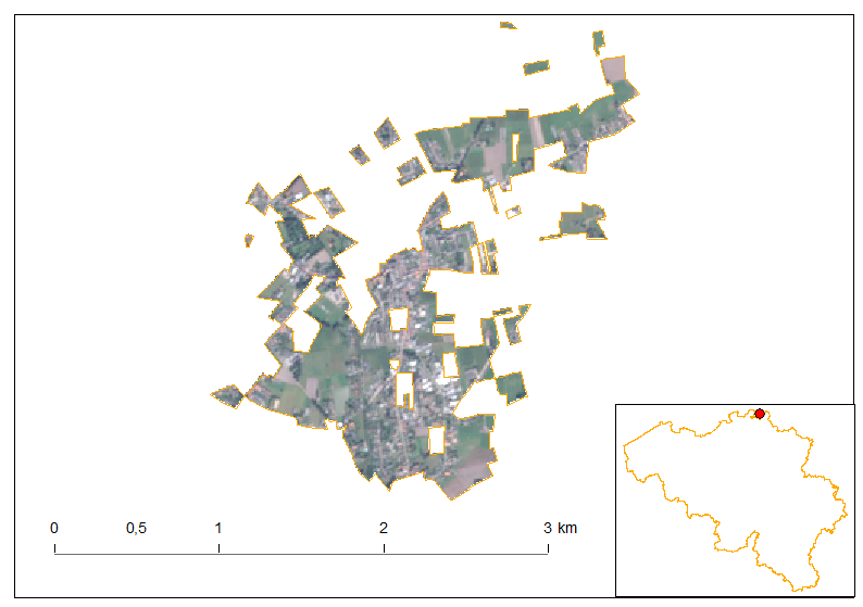
The several bassins we’re seeing here is a sign of industrial activities. Most of the waterbodies are not used anymore and were transformed into recreative facilities. Lots of campings and holiday villages are located around some of the waterbodies. Paradoxally, the town of Dessel just in the North West of the view here hosts several nuclear facilities.
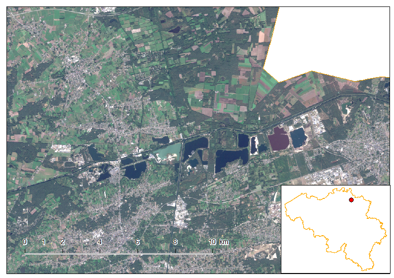
Another administrative border anomality lies in the Eastern part of Belgium. There are small corridors of Belgian land in Germany. How come? Discover it here. This part of Belgium is also where the highest point above the sea level lies: Signal de Botrange at 694m above Sea level. A lot of green areas are visible as the region is very densily forested. The two water bodies in the North of the image area, in the West, the barrage of the Gilpesse, and, in the East, the Barrage of Eupen.
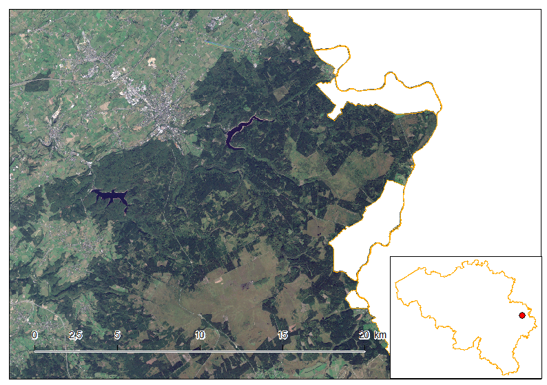
Another big miritime port in Belgium is the port of Zeebrugge. The portuar infrastruture extends ways beyond the coast (up to 3.5km into the North Sea). In the North East there is the chic coastal village of Knokke-Heist, known for being the Belgian’s St Tropez.
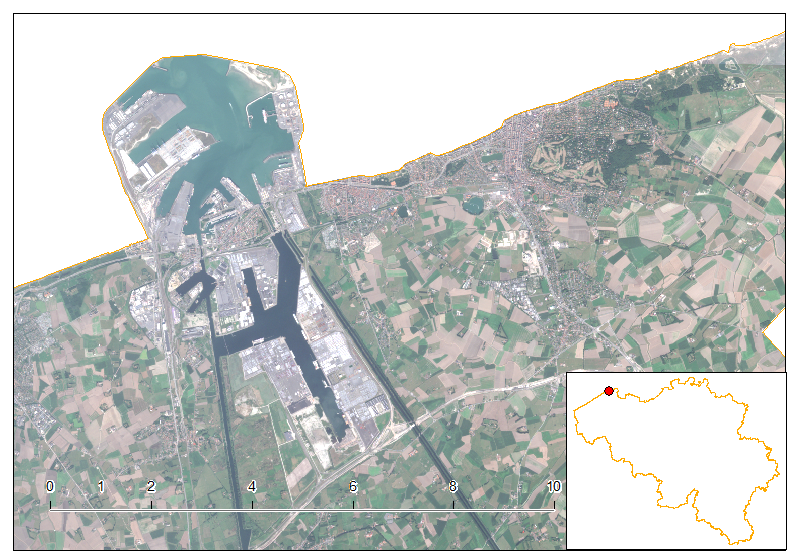
The lakes of l’Eau d’Heure is composed of 5 artifial waterbodies, which stretches over 600ha. This place is known for the watersports and fishing facilities. It is located at the South of the Province of Hainaut, but also partly in the Province of Namur.
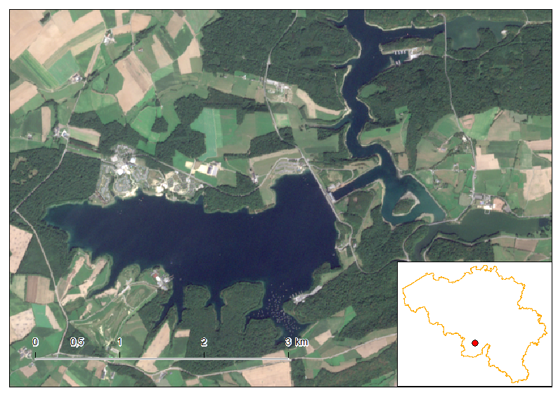
Belgium has an important space industry since decades. The area pictured here is a field of parabolic antenna which mission is to make the link between terrestrial and space communications. The village just above the antenna field is Lessive and not so far away lies the Euro Space Center, a business area deploying top notch space-related companies.
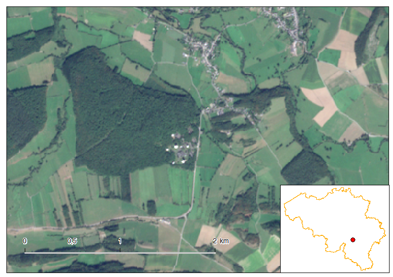
The Semois river flows not far away from the Belgian-French border. The numerous curves translate the rock and soil composition, mainly schist, as the river cuts its bed in the direction of the sheet-shaped underlying rock structure. Numerous idyllic villages are located in, or nearby, the Semois course and the most notable is Bouillon just a few kilometers from here.
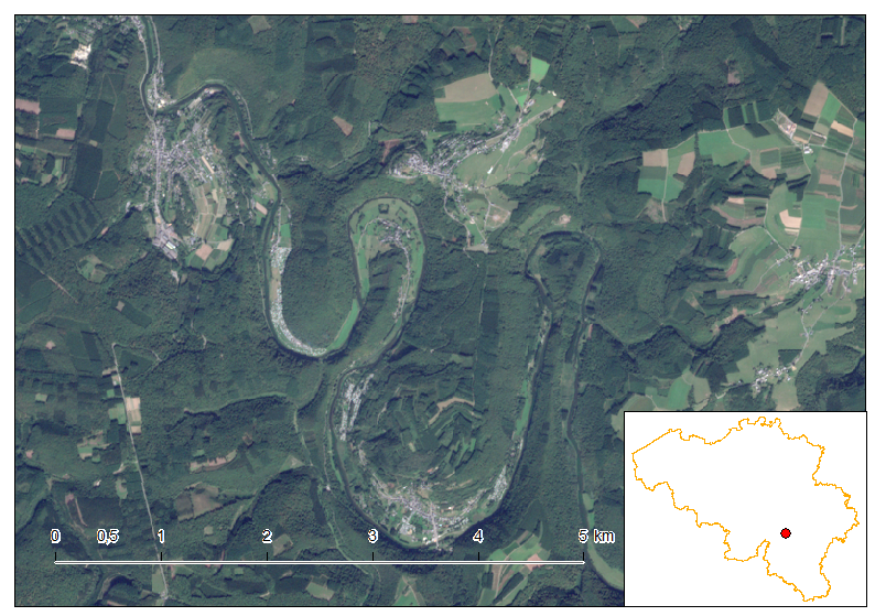
An abandoned meander, forming here an oxbow lake, is visible here near the town of Dendermonde. The river is the Scheldt, the same as the one that flows into the sea in Antwerp.
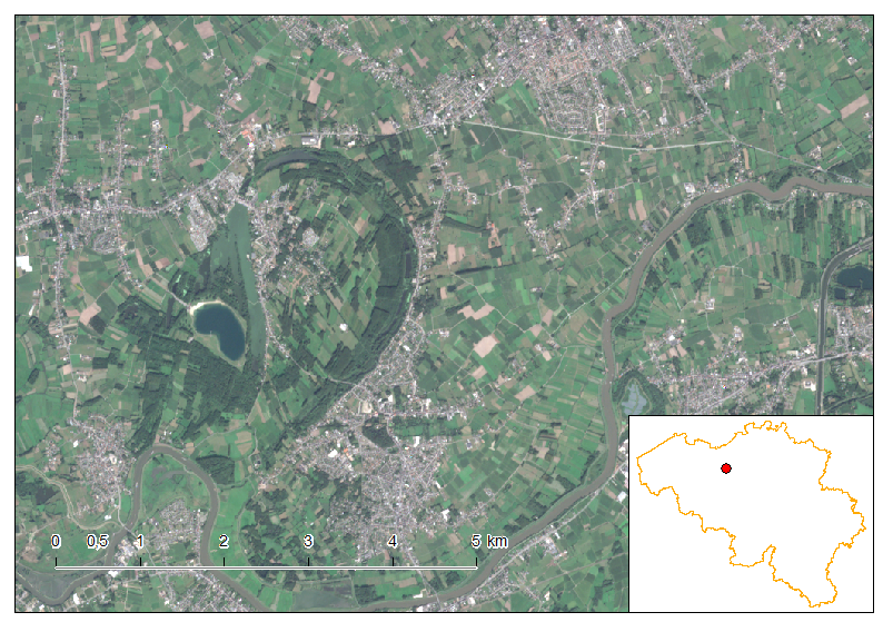
The journey accross Belgium would have been complete without a space view of Brussels, the capital of Belgium and home of most of the European Union institutions. Downtown is located in the West inside of the pentagon shaped road network. The European institutions are more in the center and in the East, near the parc du centenaire. Brussels is one of the capital in the worl where there are the most green spaces.
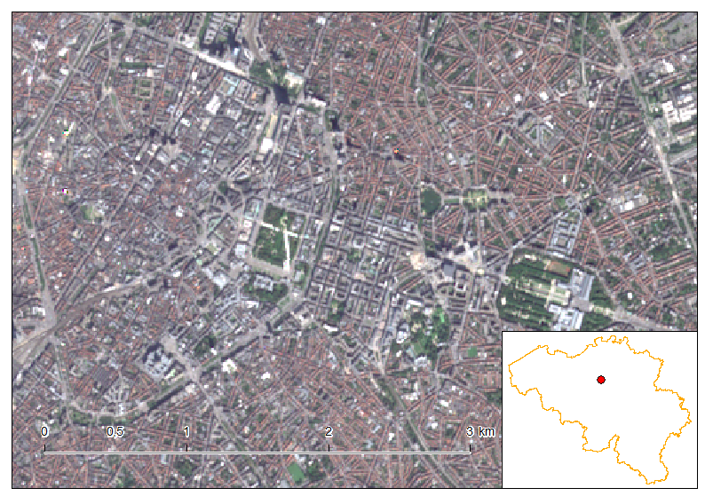
Belgium developped in the 70’s nuclear energy provisions, with the construction of the nuclear power plant of Tihange here, and another one in Doel, near Antwerp. The chemneys are visible in the North where only one is producing clouds. Tihange is very near to the town of Huy, which is in the West inside the curve of the Meuse River.
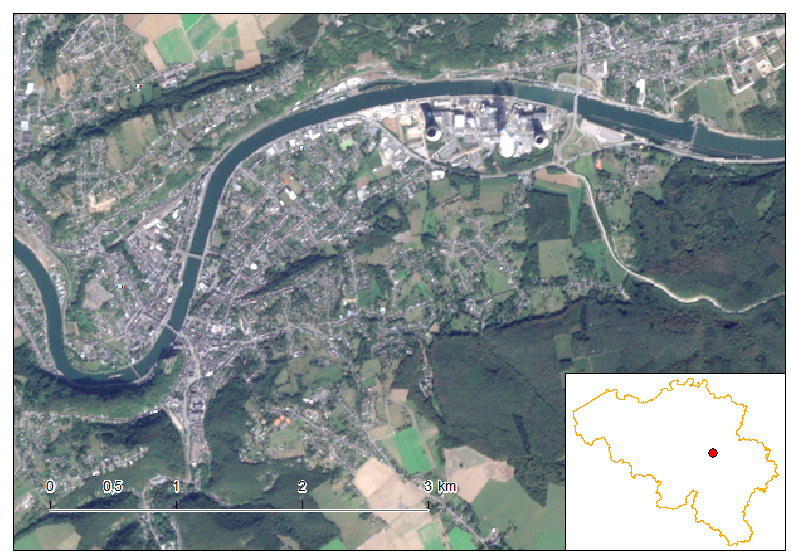
Belgium has much more to offer than just these 15 places described here. The article would have been far too long if all the beautiful places would have been described.
I hope you enjoyed this small Sentinel-2 journey accorss Belgium and I hope the images of Belgium is much more brighter to you than just reduced to Belgian (!) Fries and chocolate eaters.
Cheers,
Daniel
Full recipe to reproduce at home
Full recipe to reproduce at home, provided you have a valid ArcGIS for Desktop license.
I am used to use python scripting as much as I can. This gives me more control of the geoprocessing rather than using a UI.
For this mosaic, I used the following granules (see this article to get the granules):
31UDS_20160921
31UFS_20160925
31UER_20160908
31UES_20160908
31UET_20160401
31UFQ_20160826
31UFR_20160925
31UGS_20160925
31UFT_20160925
31UGR_20160925
First, we go through a set of imports of the original Sentinel-2 jp2 images into the gdb format. Repeat this procedure 9 times for each of the granules.
import arcpy
arcpy.RasterToGeodatabase_conversion(['<PATH_TO_DATA>\\IMG_DATA\\B01.jp2',
'<PATH_TO_DATA>\\IMG_DATA\\B02.jp2', '<PATH_TO_DATA>\\IMG_DATA\\B03.jp2',
'<PATH_TO_DATA>\\IMG_DATA\\B04.jp2', '<PATH_TO_DATA>\\IMG_DATA\\B05.jp2',
'<PATH_TO_DATA>\\IMG_DATA\\B06.jp2', '<PATH_TO_DATA>\\IMG_DATA\\B07.jp2',
'<PATH_TO_DATA>\\IMG_DATA\\B08.jp2', '<PATH_TO_DATA>\\IMG_DATA\\B09.jp2',
'<PATH_TO_DATA>\\IMG_DATA\\B10.jp2', '<PATH_TO_DATA>\\IMG_DATA\\B11.jp2',
'<PATH_TO_DATA>\\IMG_DATA\\B12.jp2', '<PATH_TO_DATA>\\IMG_DATA\\B8A.jp2'], r'<PATH_TO_GDB>\WHOLE_BELGIUM.gdb')
arcpy.Rename_management(r'<PATH_TO_GDB>\WHOLE_BELGIUM.gdb\B01', 'B01_01')
arcpy.Rename_management(r'<PATH_TO_GDB>\WHOLE_BELGIUM.gdb\B02', 'B02_01')
arcpy.Rename_management(r'<PATH_TO_GDB>\WHOLE_BELGIUM.gdb\B03', 'B03_01')
arcpy.Rename_management(r'<PATH_TO_GDB>\WHOLE_BELGIUM.gdb\B04', 'B04_01')
arcpy.Rename_management(r'<PATH_TO_GDB>\WHOLE_BELGIUM.gdb\B05', 'B05_01')
arcpy.Rename_management(r'<PATH_TO_GDB>\WHOLE_BELGIUM.gdb\B06', 'B06_01')
arcpy.Rename_management(r'<PATH_TO_GDB>\WHOLE_BELGIUM.gdb\B07', 'B07_01')
arcpy.Rename_management(r'<PATH_TO_GDB>\WHOLE_BELGIUM.gdb\B08', 'B08_01')
arcpy.Rename_management(r'<PATH_TO_GDB>\WHOLE_BELGIUM.gdb\B09', 'B09_01')
arcpy.Rename_management(r'<PATH_TO_GDB>\WHOLE_BELGIUM.gdb\B10', 'B10_01')
arcpy.Rename_management(r'<PATH_TO_GDB>\WHOLE_BELGIUM.gdb\B11', 'B11_01')
arcpy.Rename_management(r'<PATH_TO_GDB>\WHOLE_BELGIUM.gdb\B12', 'B12_01')
arcpy.Rename_management(r'<PATH_TO_GDB>\WHOLE_BELGIUM.gdb\B8A', 'B8A_01')
Create then a distinct mosaic dataset for each of the bands. Here’s the example for Band n°1, and repeat the process for bands 2, 3 until 12 (do not forget band n°8A!).
arcpy.CreateMosaicDataset_management(in_workspace="<PATH_TO_GDB>/WHOLE_BELGIUM.gdb",
in_mosaicdataset_name="B01", coordinate_system="PROJCS['Belge_Lambert_2008',GEOGCS['GCS_ETRS_1989',DATUM['D_ETRS_1989',
SPHEROID['GRS_1980',6378137.0,298.257222101]],PRIMEM['Greenwich',0.0],UNIT['Degree',0.0174532925199433]],
PROJECTION['Lambert_Conformal_Conic'],PARAMETER['False_Easting',649328.0],PARAMETER['False_Northing',665262.0],
PARAMETER['Central_Meridian',4.359215833333333],PARAMETER['Standard_Parallel_1',49.83333333333334],
PARAMETER['Standard_Parallel_2',51.16666666666666],PARAMETER['Latitude_Of_Origin',50.797815],
UNIT['Meter',1.0]];-35373000 -30122500 10000;-100000 10000;-100000 10000;0,001;0,001;0,001;IsHighPrecision",
num_bands="", pixel_type="", product_definition="NONE", product_band_definitions="")
Add then the bands to the mosaic. (to do for all the layers)
arcpy.AddRastersToMosaicDataset_management(in_mosaic_dataset="<PATH_TO_GDB>/WHOLE_BELGIUM.gdb/B01",
raster_type="Raster Dataset", input_path="<PATH_TO_GDB>\\WHOLE_BELGIUM.gdb\\B01_01;
<PATH_TO_GDB>\\WHOLE_BELGIUM.gdb\\B01_02;
<PATH_TO_GDB>\\WHOLE_BELGIUM.gdb\\B01_03;
<PATH_TO_GDB>\\WHOLE_BELGIUM.gdb\\B01_04;
<PATH_TO_GDB>\\WHOLE_BELGIUM.gdb\\B01_05;
<PATH_TO_GDB>\\WHOLE_BELGIUM.gdb\\B01_06;
<PATH_TO_GDB>\\WHOLE_BELGIUM.gdb\\B01_07;
<PATH_TO_GDB>\\WHOLE_BELGIUM.gdb\\B01_08;
<PATH_TO_GDB>\\WHOLE_BELGIUM.gdb\\B01_09;
<PATH_TO_GDB>\\WHOLE_BELGIUM.gdb\\B01_10;
",update_cellsize_ranges="UPDATE_CELL_SIZES", update_boundary="UPDATE_BOUNDARY",
update_overviews="NO_OVERVIEWS", maximum_pyramid_levels="", maximum_cell_size="0",
minimum_dimension="1500", spatial_reference="", filter="#", sub_folder="SUBFOLDERS",
duplicate_items_action="ALLOW_DUPLICATES", build_pyramids="NO_PYRAMIDS", calculate_statistics="NO_STATISTICS",
build_thumbnails="NO_THUMBNAILS", operation_description="#", force_spatial_reference="NO_FORCE_SPATIAL_REFERENCE")
The mosaic are then exported to raster dataset into a gdb (do it for all of the mosaic/bands).
arcpy.MosaicToNewRaster_management(input_rasters="<PATH_TO_GDB>/WHOLE_BELGIUM.gdb/B01",
output_location="<PATH_TO_GDB>/WHOLE_BELGIUM.gdb", raster_dataset_name_with_extension="BELGIUM_B01",
coordinate_system_for_the_raster="", pixel_type="16_BIT_UNSIGNED", cellsize="",
number_of_bands="1", mosaic_method="LAST", mosaic_colormap_mode="FIRST")
Finally we have to clip the final results to only keep pixels inside the Belgium territory (for that, we need a Belgium layer with the exact national extent).
arcpy.Clip_management(in_raster="<PATH_TO_GDB>/WHOLE_BELGIUM.gdb/BELGIUM_B01",
rectangle="522281,353430353 521165,124731085 795172,027834512 744030,366077007",
out_raster="<PATH_TO_GDB>/WHOLE_BELGIUM.gdb/BELGIUM_B01_Clip",
in_template_dataset="<PATH_TO_GDB>/WHOLE_BELGIUM.gdb/BELGIUM", nodata_value="65536",
clipping_geometry="ClippingGeometry", maintain_clipping_extent="NO_MAINTAIN_EXTENT")
Agriculture and Sentinel-2: An unsupervised temporal classification
September 1st, 2016Remote Sensing and agriculture always have been best friends. With the arrival of Sentinel-2 data, the friendship got even more stronger! In this article, we’re trying to figure out how we could use Sentinel-2 data to make an unsupervised crop parcel classification. With a reference image by side, we then determine the crop types. The study area is in the UTM Zone 31UFS (Belgium).
Our goal in this article is to identify different agricultural crop parcels using temporal satellite imageries by applying an unsupervised classification. Agricultural parcels look different depending on the season we’re looking at. Land is usually naked during winter and crops commence their growth in early Spring. The growth peak is around May, June or July for most of the cultures but some others are highest in August or September. Doing a classification on a unique scene will not be suitable as all bare lands will look the same (even if they later differentiate depending on the crop type).
The images on which we do the classification were taken at two different periods. Sentinel-2 scenes are composed of 13 different bands of different resolutions. The crop types, and all the land in general, thus have a different spectral signature. The more bands they are, the easier the differentiation between two crop types will be. Merging both scenes into one and unique document having a total of 20 bands, leaving by side the 60-m resolution bands 1-9-10, will make the differenciation even more relevant. Notice also that two bare land parcels looking the same at the same period are thus not considered as being of the same crop type when they have different spectral signature at another moment.
We decided to make a temporal unsupervised classification using satellite images on two different moments: One was taken the 21th of April 2016, the other the 26th of August 2016.
Here are the steps we followed. Note that I use ArcGIS for Desktop with the Spatial Analyst extension.
- Data acquisition (21/04/2016 and 26/08/2016)
- Band composition
- Unsupervised classification
- Crop identification using a reference document (official SPW document)
Data acquisition
The Sentinel-2 data can be acquired using the Sentinels Scientific Data Hub or using the open Sentinel-2 on AWS service (preferred method). From the AWS service webpage, use the interactive data search application. Zoom to the area of interest, specify the data and the cloud coverage, and go on the tile data link page.
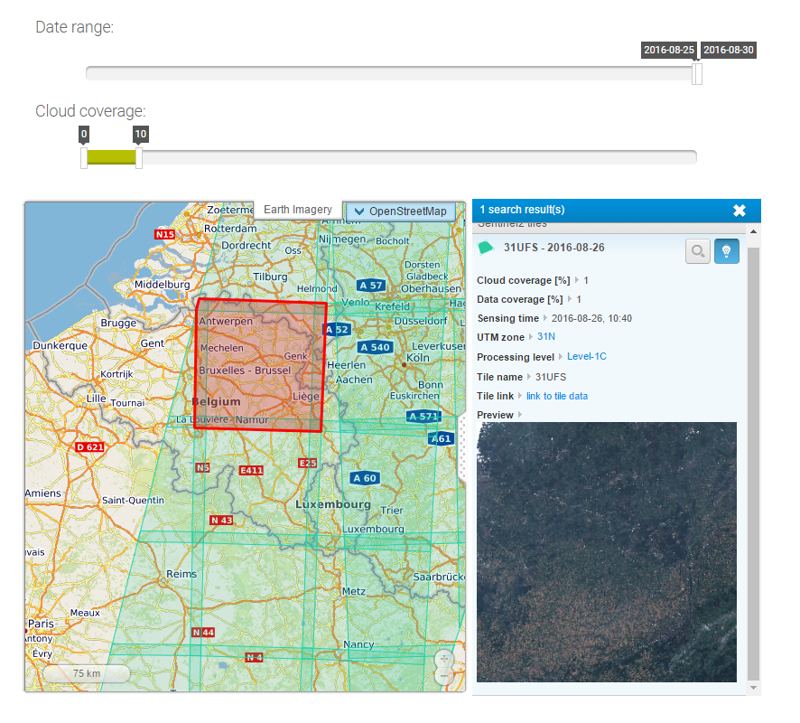
Sentinel-2 data service on AWS
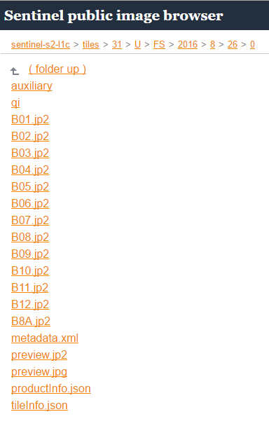
Sentinel 2 data structure
The dates are not chosen randomly: we need to have a minimum cloud cover percentage. The document of the 21st of April is the best one during the considered growing season. Fortunately, the last scene available (26th of August) is cloud free.
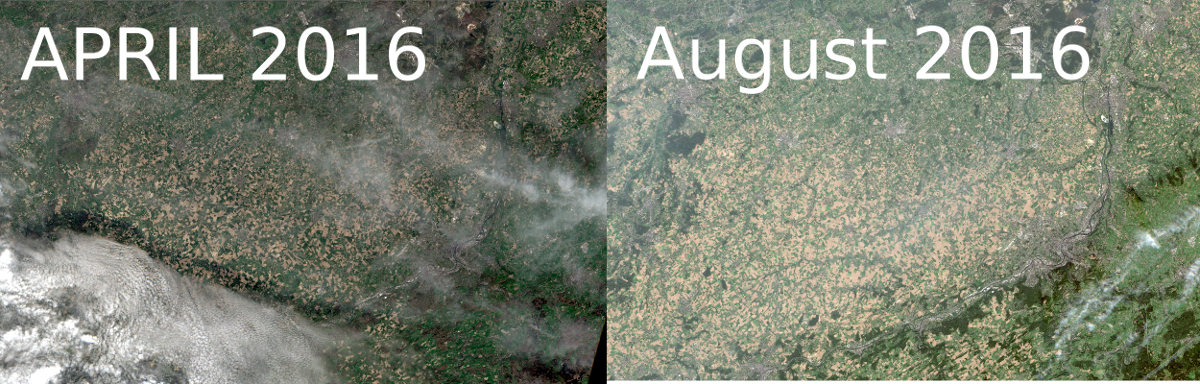
Band composition
As said, we want, first, to create a unique scene composed of 20 bands. Using ArcGIS for Desktop, we use the Composite Bands tool. As input, we specify all the layers B02.jp2, B03.jp2, etc. but not B01.jp2, B09.jp2 and B11.jp2. These bands corresponds respectively to the aerosol band, water vapour and cirrus bands. We exclude them because their resolution is about 60m, which is the highest of all the bands considered.
Unsupervised classification
The unsupervised classification is done straighforward. Activate the Spatial Analyst extension and add the Spatial Analyst toolbar to the menu.
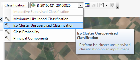
Click on the Iso Cluster Unsupervised Classification feature and specify 35 as the number of output classes (remember, the scenes represent an area of 100x100km).
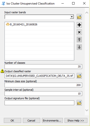
ISOCLUSTER
Here’s the raw result in greayscale.

Raw unsupervised classification
We need now to clean up this result. This image contains a lot of speckles that we need to clean up. Also, there are lots of areas which are so small around other areas that we need to delete.
We run the Majority Filter that assign to isolated pixels the pixel of their more frequent neighbors.
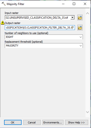
MAJORITY FILTER
And then a Boundary Clean operation.
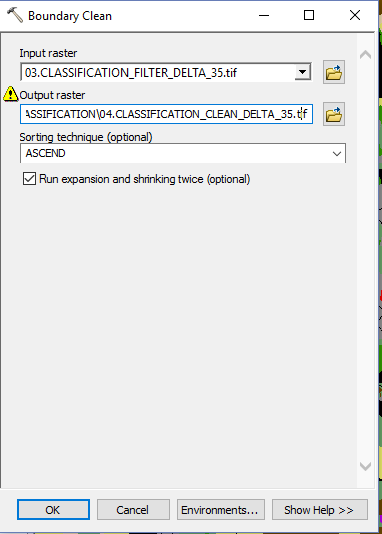
BOUNDARY CLEAN
The Region Group processing groups together pixels that have the same values. After this operation, we have the 35 classes cleaned up. Attention however as small areas such as isolated pixels, isolated and small pixel corridors, etc. can remain in the image. We now clean this up as we first need to define a threshold from which we consider removing the area
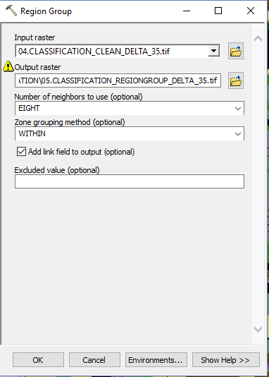
REGION GROUP
We use the Set Null operation where we consider that areas of less than 40 pixels are removed.
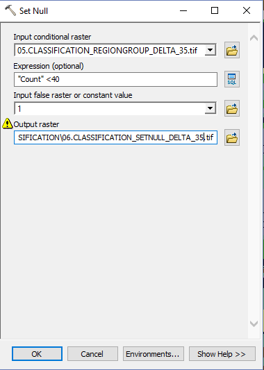
Set Null operation
The last operation is Nibble. As input, we take into account the mask that we just define with the Set Null operation and the cleaned unsupervised image (coming out from the Boundary Clean operation).
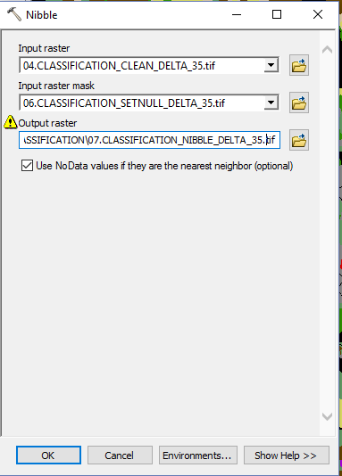
NIBBLE
Crop identification
We finally got our clean classification result! The last thing to do is to add a reference layer in order to identify the crops. The same areas on both the reference layer and our classification are supposed to be of the same type. Notice however that we discovered some differences and we see two main reasons:
- Our classification is based on 2016 imageries whereas the reference document is from 2015. It is possible that crop type change from one year to another
- Our technique to identify the same crop types is not optimal (similar spectral signatures from different crop type, too broad temporal resolution and not enough images taken into account (April – August), etc.)
As we are in Belgium and mostly in the Walloon Region, we can take a ready to use layer provided by the SPW (Service Public de Wallonie).
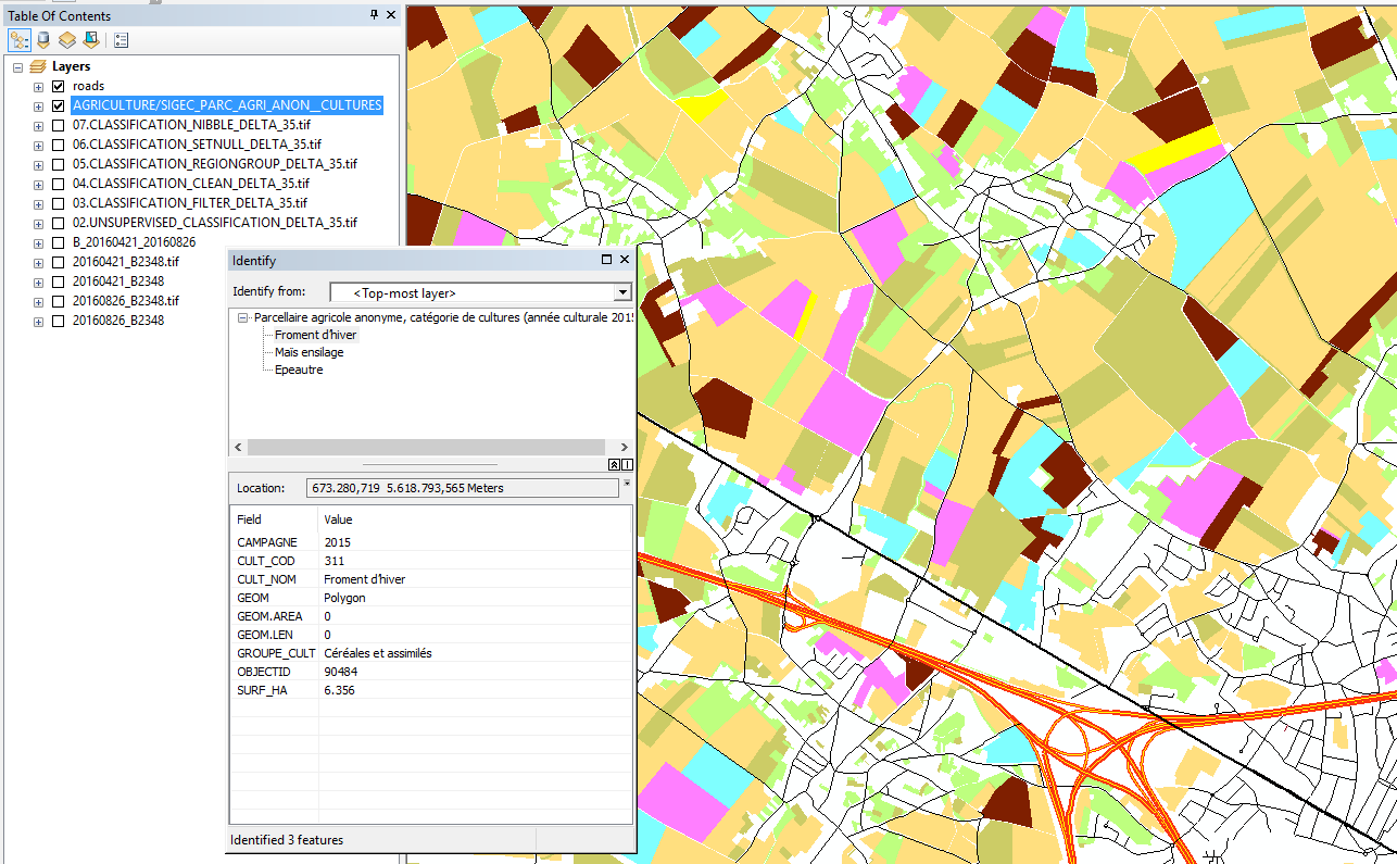
REFERENCE LAYER
Here is our final result.
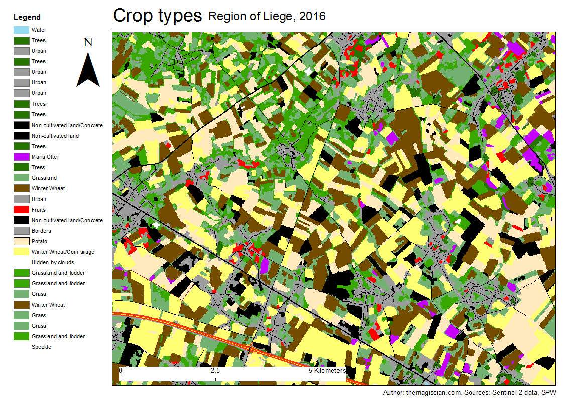
Agriculture classification
Conclusion
We’ve seen that with the two provided Sentinel-2 data using both 10 bands and ArcGIS for Desktop, we were able to run an unsupervised classification and to assign the detected zone to crop type using a reference image.
Cheers,
Daniel