Spatial Database battles exists since … the existence of spatial databases! Two most prominent spatial database in the GIS world are Oracle Spatial and PostgreSQL/PostGIS, both having advantages and disadvantages.

While most of the GIS customers are still using file-based data – we are all guilty because we ALL still use Shapefiles – the trends show that more organizations are moving to centralized systems involving spatial databases, more than ever before. Spatial databases offer a lot of advantages file-based system do not have. Here are a few of them (Source). They:

• Handle data more efficiently
• Are better performant
• Are better integrated with external applications
• Take up less space
• Have reduced redundancy risks
• Benefit of the power of SQL with which you can theoretically do anything with the data
• You have more control on the data and processing are less black-boxed
• …

On the other hand, they have a big disadvantage towards file-based systems: they require skills for the implementation, maintenance, usage, etc. (themagiscian.com can help 🙂 ). Small organizations with a few GIS experts, or not trained personal, thus have more difficulties handling bigger systems. It all comes to the need the organization have: Is it just producing maps? Does it need to be interoperable when there’s only one GIS expert in-house? Etc.

In this article, we will compare, from the technical side, PostGIS and Oracle Spatial. We won’t go into installation, configuration, and tuning – we assume we have already up and running systems – but we will only compare the differences in the spatial functions for manipulating geospatial data.

Saying Oracle is more robust than PostGIS begins to be not always true as the overall PostgreSQL community takes the performances very serious. This article shows the advantage of PostGIS over Oracle in both the cold and warm phase when it comes to performance testing. This article is also referenced by this one. Even Oracle itself recognize some best performances done by PostGIS compared to Oracle. Other tests done in March 2016 on very simple queries shows the faster PostGIS.

Let’s be clear: the goal of this article is NOT to advocate for one or the other system in the implementation of a spatial database. It all comes to the purpose of such an implementation, the budget, the goals, etc. We’re just comparing the way the requests are built for doing basic spatial operations.

The exercices are about the handling of data about the municipalities in Belgium for the vectors and a Sentinel-2 scene to illustrate basic tasks for rasters.

Let’s go!

1. Connection as “root”

PostGIS

The command line client is psql

psql -Upostgres -h<ip>

Oracle Spatial

In Oracle, we use sqlplus

sqlplus sys/oracle@<ip>:1521/orcl as sysdba

2. Create User/Schema

PostGIS

Our user “daniel” is created following way

CREATE USER daniel WITH PASSWORD 'daniel';

Oracle Spatial

In Oracle, the concept of user and schema is very different from what it is in PostGIS. We have to see the schema as a user account with all the objects and tables associated with it. We need to add an additional clause to give the basic priviledges to our user

CREATE USER daniel IDENTIFIED BY daniel DEFAULT TABLESPACE daniel_ts;
GRANT CONNECT, RESOURCE TO daniel;

3. Create Spatial Database

PostGIS

In PostGIS, for each database created, we have to enable the spatial extension of the table for all the tables

CREATE DATABASE daniel WITH OWNER daniel;
CREATE EXTENSION postgis;

Oracle Spatial

Nothing to do! What? Yes nothing to do! In the previous step we create a user/schema, which is in fact a set of objects composed of user, objects, tables, views, triggers.

4. Import a Shapefile

PostGIS

For PostGIS, we use the shp2pgsql tool provided with the PostGIS installation. Let’s import our Belgian municipalities shapefile

shp2pgsql -s3812 -d -ggeom -I "[DATAPATH]\Municipalities_A_AdMu.shp" public.a_municipalities 
| psql -Udaniel -h<ip> -ddaniel

Oracle Spatial

For Oracle, three methods are at our disposal.

The first being the use of Java classes and the librarie provided by a client instance

java -classpath %ORACLE_HOME%\jdbc\lib\ojdbc7.jar;%ORACLE_HOME%\md\lib\sdoutl.jar;
%ORACLE_HOME%\md\lib\sdoapi.jar oracle.spatial.util.SampleShapefileToJGeomFeature 
-h <ip> -p 1521 -s orcl -u daniel -d daniel -t municipalities 
-f "[DATAPATH]\Municipalities_A_AdMu.shp" -r 3812 -g geom

The second solution is the use of the ogr2ogr utility

ogr2ogr -progress -lco SRID=3812 -lco GEOMETRY_NAME=geom -nlt MULTIPOLYGON 
-nln a_municipalities -f "OCI" -overwrite OCI:daniel/daniel@<ip>/orcl "[DATAPATH]\Municipalities_A_AdMu.shp"

The third solution is using the mapbuilder tool and thus manually uploading the shapefile.

Note that the ogr2ogr for Oracle is much more picky than the shp2pgsql tool for PostGIS. You may have to play with the different import options as every single discrepancy in the shapefile will reject the whole feature during the data loading phase. Be sure the Shapefile is PERFECT!

5. Feature count

PostGIS

This is an easy one

SELECT count(*) FROM a_municipalities;
 count
-------
 589
(1 row)

We have 589 municipalities in Belgium, which is correct.

Oracle Spatial

SELECT count(*) FROM a_municipalities;
 COUNT(*)
----------
 589

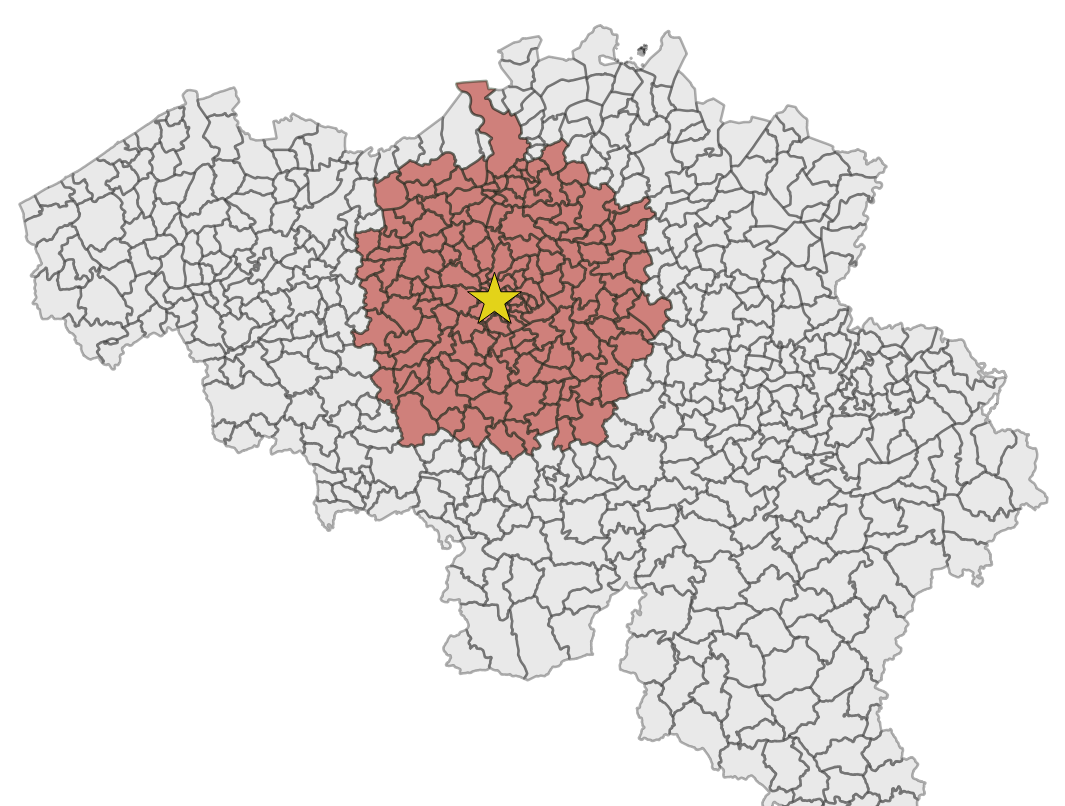
6. Get the list of municipalities which are in a radius of 30 km from Brussels, the capital

PostGIS

We use the ST_DWithin function in the WHERE clause

SELECT m2.admunafr FROM a_municipalities m1, a_municipalities m2 
WHERE m1.admunafr = 'BRUXELLES' AND ST_DWithin(m1.geom, m2.geom, 30000);

Oracle Spatial

In Oracle Spatial we make use of the SDO_WITHIN_DISTANCE function from the SDO_GEOM package

SELECT m2.admunafr FROM a_municipalities m1, a_municipalities m2 
WHERE m1.admunafr = 'BRUXELLES' AND SDO_WITHIN_DISTANCE(m1.geom, m2.geom, 'distance=30000') = 'TRUE' ;

Both results return the same set.

7. Getting the biggest municipality

PostGIS

Usage of the ST_Area function (the units of the result is in km²)

SELECT admunafr, area FROM (
    SELECT admunafr, ST_Area(geom)/1000000 area FROM a_municipalities) t 
ORDER BY area desc LIMIT 1;

 admunafr | area
----------+------------------
 TOURNAI | 215.367669469211
(1 row)

Oracle Spatial

Usage of the SDO_AREA function of the SDO_GEOM package. A little bit longer as we have to keep only the first result from the resulting table.

SELECT admunafr, area FROM 
     (SELECT admunafr, area FROM 
          (SELECT admunafr, SDO_GEOM.SDO_AREA(geom, 0.0005)/1000000 area 
          FROM a_municipalities) t ORDER BY area desc) u 
 WHERE rownum = 1;

ADMUNAFR AREA
------------------------ ----------
TOURNAI 215,367669

8. Get the 5 municipalities with the most neighbours

PostGIS

We use the function ST_Touches in the WHERE clause and when two municipalities touches, we count 1. The resulting table is then grouped and the ‘1’ summed.

SELECT admunafr, sum(count) neighbours FROM 
     (SELECT m1.admukey, m1.admunafr, 1 count FROM a_municipalities m1, a_municipalities m2 
     WHERE m1.objectid != m2.objectid AND ST_Touches(m1.geom, m2.geom)) t 
GROUP BY admukey, admunafr ORDER BY neighbours DESC LIMIT 5;
 admunafr | neighbours
-----------+------------
 BRUXELLES | 16
 ANVERS | 14
 GAND | 12
 LIEGE | 11
 TONGRES | 11
(5 rows)

No surprise, they are mostly big cities with Brussels having a total of 16 neighbouring municipalities! For your information, here are they

SELECT m2.admunafr FROM a_municipalities m1, a_municipalities m2 WHERE m1.objectid != m2.objectid 
AND ST_Touches(m1.geom, m2.geom) AND m1.admunafr = 'BRUXELLES' ORDER BY m2.admunafr;

admunafr
-----------------------
 ANDERLECHT
 ETTERBEEK
 EVERE
 GRIMBERGEN
 IXELLES
 JETTE
 MACHELEN
 MOLENBEEK-SAINT-JEAN
 SAINT-GILLES
 SAINT-JOSSE-TEN-NOODE
 SCHAERBEEK
 UCCLE
 VILVORDE
 WATERMAEL-BOITSFORT
 WEMMEL
 ZAVENTEM
(16 rows)

Oracle Spatial

For Oracle, we use the SDO_RELATE operator with the ‘touch‘ mask

SELECT admunafr, neighbours FROM 
     (SELECT admunafr, sum(count) neighbours FROM 
          (SELECT m1.admukey, m1.admunafr, 1 count FROM a_municipalities m1, a_municipalities m2 
               WHERE m1.objectid != m2.objectid AND SDO_RELATE(m1.geom, m2.geom, 'mask=touch') = 'TRUE') t 
     GROUP BY admukey, admunafr ORDER BY neighbours DESC) u 
WHERE rownum <=5;

ADMUNAFR NEIGHBOURS
------------------------ ----------
BRUXELLES 16
ANVERS 14
GAND 12
LIEGE 11
TONGRES 11

9. Municipality with longest border (perimeter)

PostGIS

The ST_Perimeter comes into play! (Again, the unit of the result is in km)

SELECT admunafr, perimeter FROM 
     (SELECT admunafr, ST_Perimeter(geom)/1000 perimeter FROM a_municipalities) t 
ORDER BY perimeter desc LIMIT 1;

 admunafr | perimeter
----------+-----------------
 TOURNAI | 103.241775546157
(1 row)

Tournai, again, has the longest border

Oracle Spatial

The SDO_LENGTH function takes the perimeter here

SELECT admunafr, perimeter FROM (SELECT admunafr, perimeter FROM 
     (SELECT admunafr, SDO_GEOM.SDO_LENGTH(geom, 0.0005)/1000 perimeter 
     FROM a_municipalities) t ORDER BY perimeter desc) u 
WHERE rownum = 1;
ADMUNAFR PERIMETER
------------------------ ----------
TOURNAI 103,241776

10. Most and Least compact municipalities

PostGIS

The compactness of a geometry, in this case the shapes of the municipalities, can have different definitions. In this case, we take the formula corresponding to the area of the municipalitiy DIVIDED by the area of the Circle having the same perimeter. A perfect circle would have a value of 1 and the least compact shape a value near to 0. We thus use here a formula in our query. Notice how we make use of the ST_Perimeter function seen before. From the area of a circle formula, which is R² * pi, and from the perimeter function, which is 2R * pi, we know that the area of an equivalent circle would be Perimeter² / pi.

SELECT admunafr, compactness FROM
     (SELECT admunafr, ST_Area(geom)/(ST_Perimeter(geom)^2 / pi() ) compactness FROM a_municipalities) t
ORDER BY compactness DESC LIMIT 5;

admunafr | compactness
 -------------+-------------------
 MERKSPLAS | 0.171412046968982
 ARENDONK | 0.165099170160105
 LOMMEL | 0.158076966995777
 RIJKEVORSEL | 0.155705115550531
 BRASSCHAAT | 0.154077135253196
 (5 rows)

We see indeed that the shapes of the selected municipalities approaches circles.

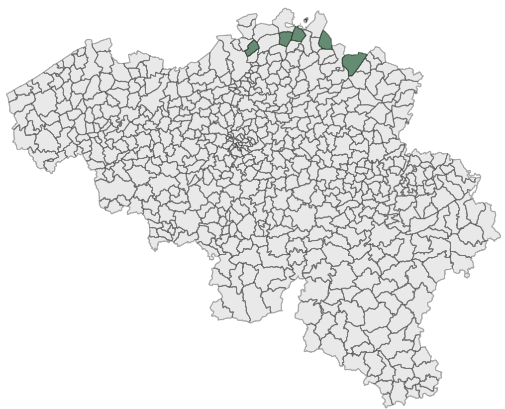
SELECT admunafr, compactness FROM (SELECT admunafr, ST_Area(geom)/(ST_Perimeter(geom)^2 / pi() ) compactness 
FROM a_municipalities) t ORDER BY compactness ASC LIMIT 5;

admunafr | compactness
 ------------+---------------------
 BAERLE-DUC | 0.00698767111042899
 RAEREN | 0.0269921358361835
 BRUXELLES | 0.0309352964504475
 WAIMES | 0.0364562022393661
 VISE | 0.0364980110812303
 (5 rows)

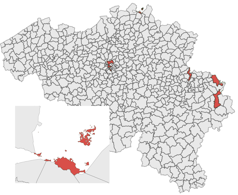
Notice how these results are coherent. The most compact municipalities are approaching circles while the least compact municipalities are much more stretched, or complicated for the municipality of Baarle-Hertog.

Oracle Spatial

Not much different formulas, but different notation. Notice: there are still no PI value constant in Oracle! We have to hard code the value 3.1415926

SELECT admunafr, compactness FROM (SELECT admunafr, SDO_GEOM.SDO_AREA(geom, 0.005)
     /(POWER(SDO_GEOM.SDO_LENGTH(geom, 0.005), 2) / 3.1415926 ) compactness 
     FROM a_municipalities ORDER BY compactness DESC) t WHERE rownum <= 5;
SELECT admunafr, compactness FROM (SELECT admunafr, SDO_GEOM.SDO_AREA(geom, 0.005)
     /(POWER(SDO_GEOM.SDO_LENGTH(geom, 0.005), 2) / 3.1415926 ) compactness 
     FROM a_municipalities ORDER BY compactness ASC) t WHERE rownum <= 5;

11. Polygons

PostGIS

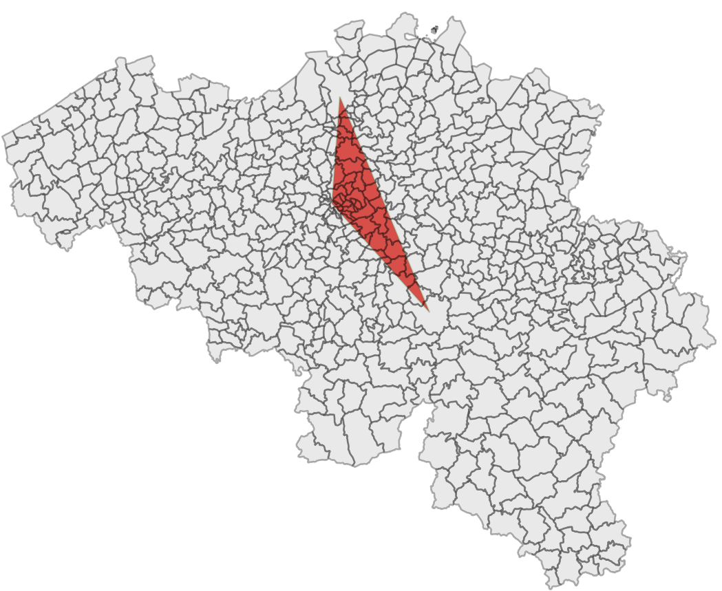
We first create the table, then we use the ST_SetGeomFromText function to insert our point. Notice: We construct a triangle where the points are the city centers of Antwerp, Brussels and Namur.

DROP TABLE f_polygons;
CREATE TABLE f_polygons (
     id serial PRIMARY KEY,
     description varchar(32),
     geom GEOMETRY(POLYGON, 3812)
);

INSERT INTO f_polygons(description, geom) VALUES ('First Polygon', 
     ST_Transform(
          ST_SetSRID(
               ST_GeometryFromText(
                    'POLYGON((4.4033 51.21972, 4.348611 50.85028, 4.867222 50.46667, 4.4033 51.21972))'), 
                         4326), 3812));

We have the coordinates in 4326 lon, lat but we need them in 3812 (Belgian Lambert 2008). ST_Transform is use for doing the reprojection. The way the geometry is described is the WKT format, an OGC standard. The last point has to be repeated to close the boundary linestring.

Oracle Spatial

DROP TABLE f_polygons;
CREATE TABLE f_polygons (
 id NUMBER GENERATED BY DEFAULT ON NULL AS IDENTITY,
 description varchar(32),
 geom SDO_GEOMETRY
 );

ALTER TABLE f_polygons ADD (
 CONSTRAINT polygons_pk PRIMARY KEY (id)
 );

INSERT INTO f_polygons(description, geom) VALUES ('First Polygon', SDO_CS.TRANSFORM(
MDSYS.SDO_GEOMETRY(
2003,
4326,
NULL,
MDSYS.SDO_ELEM_INFO_ARRAY(1,1003,1),
MDSYS.SDO_ORDINATE_ARRAY(4.4033, 51.21972, 4.348611, 50.85028, 4.867222, 50.46667, 4.4033, 51.21972)
), 3812));

DELETE FROM USER_SDO_GEOM_METADATA WHERE TABLE_NAME = 'F_POLYGONS';
INSERT INTO USER_SDO_GEOM_METADATA (TABLE_NAME, COLUMN_NAME, DIMINFO, SRID) 
VALUES (
 'F_POLYGONS', 
 'GEOM',
 SDO_DIM_ARRAY (
 SDO_DIM_ELEMENT('Long', -180, 180, 0.5),
 SDO_DIM_ELEMENT('Lat', -90, 90, 0.5)),
 3812);

DROP INDEX f_polygons_idx;
CREATE INDEX f_polygons_idx ON f_polygons (geom) INDEXTYPE IS MDSYS.SPATIAL_INDEX;

What the hell! All of this for creating a polygon with three points? YES! Welcome to Oracle!

No OGC, nothing clear text (see the numbers everywhere, they are keys to specify geom types…) and thus no OGC standard, and the spatial index is mandatory otherwise no spatial operation is possible. Notice also the mandatory insert into the USER_SDO_GEOM_METADATA table … A lot of things to take into account here!

For the geometry, we use the MDSYS.SDO_GEOMETRY operator with

• 2003 being for a two dimensional polygon (yes yes!)
• 4326 the srid
• NULL? Yes! In case you would like your polygon to be a point (huh?)
• SDO_ELEM_INFO_ARRAY(1,1003,1) : where the parameters are respectively for the starting offet (see the next parameter), defining an exterior polygon ring and telling the system to connect point with straight lines. OKAY!
•  And finally MDSYS.SDO_ORDINATE_ARRAY with all the coordinates we need! Important: It seems that finally they drop their constraint to specify the coordinates counterclockwise! Counterclockwise and clockwise now both work! Waow!

12. Points

PostGIS

Let’s see how it is to create points …

DROP TABLE g_points;
CREATE TABLE g_points (
     id serial PRIMARY KEY,
     description varchar(32),
     geom GEOMETRY(POINT, 3812)
);
INSERT INTO g_points(description, geom) VALUES ('First Point', ST_Transform(
     ST_SetSRID(
          ST_Point(4.348611, 50.85028), 4326), 3812));

The same workflow as for the polygons except that we use the ST_Point constructor.

Oracle Spatial

DROP TABLE g_points;
CREATE TABLE g_points (
     id NUMBER GENERATED BY DEFAULT ON NULL AS IDENTITY,
     description varchar(32),
     geom SDO_GEOMETRY
 );

ALTER TABLE g_points ADD (
     CONSTRAINT g_points_pk PRIMARY KEY (id)
);

INSERT INTO g_points(description, geom) VALUES ('First Point', 
     SDO_CS.TRANSFORM(
     MDSYS.SDO_GEOMETRY(
          2001,
          4326,
          MDSYS.SDO_POINT_TYPE(4.348611, 50.85028, NULL),
          NULL,
          NULL
 )
 , 3812
 ));

DELETE FROM USER_SDO_GEOM_METADATA WHERE TABLE_NAME = 'G_POINTS';
INSERT INTO USER_SDO_GEOM_METADATA (TABLE_NAME, COLUMN_NAME, DIMINFO, SRID) 
VALUES (
 'G_POINTS', 
 'GEOM',
 SDO_DIM_ARRAY (
 SDO_DIM_ELEMENT('Long', -180, 180, 0.5),
 SDO_DIM_ELEMENT('Lat', -90, 90, 0.5)),
 3812);

DROP INDEX g_points_idx;
CREATE INDEX g_points_idx ON g_points (geom) INDEXTYPE IS MDSYS.SPATIAL_INDEX;

Wow again! But here we use other codes in the SDO_GEOMETRY constructor. The third parameter, which was NULL for the polygons, is now filled with values for specifying a point. It is more performant to separate point and polygon creation they say.

13. Raster Import

PostGIS

Let’s see how both spatial databases handle the import of rasters. We’re using Sentinel-2 cloud-free scenes of the Belgian coast taken the 31st of October 2016.

raster2pgsql -c -C -s 32631 -f rast -F -I -M -t 100×100 [PATHTODATA]/B02.jp2 public.h_b02 | psql -Udaniel -h<ip> -ddaniel
raster2pgsql -c -C -s 32631 -f rast -F -I -M -t 100×100 [PATHTODATA]/B03.jp2 public.h_b03 | psql -Udaniel -h<ip> -ddaniel
raster2pgsql -c -C -s 32631 -f rast -F -I -M -t 100×100 [PATHTODATA]/B04.jp2 public.h_b04 | psql -Udaniel -h<ip> -ddaniel

raster2pgsql is a utility coming with the PostGIS extension. The following parameters stand for.

• -c: create the table
• -C: apply raster constraints
• -s: specify the ouput srid
• -f: specify the name of the raster column
• -F: adds a column with the name of the file
• -I: Creates the index
• -M: Vacuum raster table
• -t: specifies, in pixels, the size of the tiles in which the raster has to be cut

Oracle Spatial

In Oracle Spatial, we first need to create the welcoming raster tables! Nothing created by a potential import script!

After the creation of the tables, we need to create the raster data tables: the rdt. The first containing the raster, the other the data associated with them.

DROP TABLE h_belgium;
CREATE TABLE h_belgium(
     georid number primary key,
     source_file varchar2(80),
     description varchar2(256),
     georaster sdo_georaster,
     load_duration number,
     pyramid_duration number
);

DROP TABLE h_belgium_rdt;
CREATE TABLE h_belgium_rdt OF sdo_raster (
     PRIMARY KEY (
         rasterId, pyramidLevel, bandBlockNumber,
         rowBlockNumber, columnBlockNumber)
)
LOB (rasterblock) STORE AS SECUREFILE (NOCACHE NOLOGGING);

-- INSERT INTO USER_SDO_GEOM_METADATA
DELETE FROM user_sdo_geom_metadata WHERE table_name in ('H_BELGIUM');
INSERT INTO user_sdo_geom_metadata (
     table_name, column_name, diminfo, srid
)
VALUES (
     'H_BELGIUM',
     'GEORASTER.SPATIALEXTENT',
     sdo_dim_array(
     sdo_dim_element('LONG', 499980, 508980, 0.05),
     sdo_dim_element('LAT', 5699000, 5700000, 0.05)
     ),
 32631
);
COMMIT;

EXECUTE sdo_geor_admin.registerGeoRasterColumns;
SELECT * FROM THE (SELECT SDO_GEOR_ADMIN.listGeoRasterColumns FROM DUAL);
EXECUTE sdo_geor_admin.registerGeoRasterObjects;

Then, we can use … GDAL! You could use the GeoRasterLoader class provided with the Georaster Tools but … good luck!

gdal_translate -of georaster [PATHTODATA]\B02.jp2" georaster:daniel/daniel@<ip>:1521/orcl,H_BELGIUM,georaster 
-co blockxsize=512 -co blockysize=512 -co blockbsize=3 -co interleave=bip -co srid=32631 -co 
"insert=values(1, '31UES20161031/b02.jp2', 'H_BELGIUM S2 B02', sdo_geor.init('H_BELGIUM_RDT', 1),null,null)" -co compress=deflate
gdal_translate -of georaster [PATHTODATA]\B03.jp2" georaster:daniel/daniel@<ip>:1521/orcl,H_BELGIUM,georaster 
-co blockxsize=512 -co blockysize=512 -co blockbsize=3 -co interleave=bip -co srid=32631 -co 
"insert=values(2, '31UES20161031/b03.jp2', 'H_BELGIUM S2 B03', sdo_geor.init('H_BELGIUM_RDT', 2),null,null)" -co compress=deflate
gdal_translate -of georaster [PATHTODATA]\B04.jp2" georaster:daniel/daniel@<ip>:1521/orcl,H_BELGIUM,georaster 
-co blockxsize=512 -co blockysize=512 -co blockbsize=3 -co interleave=bip -co srid=32631 -co 
"insert=values(3, '31UES20161031/b04.jp2', 'H_BELGIUM S2 B04', sdo_geor.init('H_BELGIUM_RDT', 3),null,null)" -co compress=deflate

See how we have to initialize the rasters.

After the import, we must create the index to make the georaster fully exploitable.

-- CREATE INDEX
DROP INDEX H_BELGIUM_SX;
CREATE INDEX H_BELGIUM_SX
 ON H_BELGIUM (georaster.spatialextent)
 indextype IS mdsys.spatial_index;
COMMIT;

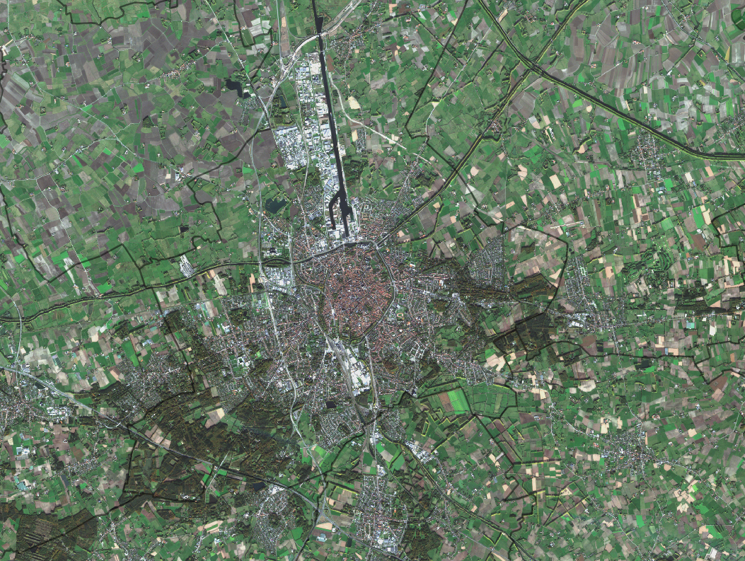
With a nice True Colour band combination, we got the following result. Example with the city of Bruges near the Belgian coast.

Conclusion

Both PostGIS and Oracle Spatial have advantages and disadvantages. PostGIS seems however easier to install, to manage and to manipulate. It is futhermore totally FREE and at the hand of every small to big business. Oracle Spatial still has a big and good reputation with a hard-working team behind the product and a proven record of robustness.

Cheers,

 

Daniel