
Posts by themagiscian:
Earthquake in Amatrice, Italy: Before/After with Sentinel-2
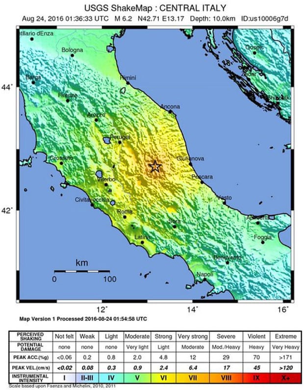
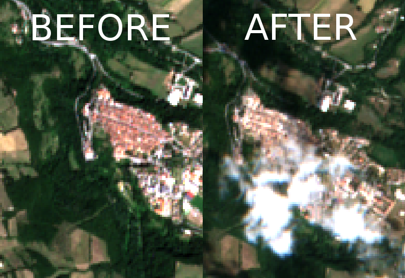
August 29th, 2016Sentinel-2 imageries can be used in a huge variety of applications. I was trying to figure out how these free data could be used in the monitoring of Earthquake damage. The case of Amatrice, Italy, where an earthquake occur early in the morning of the 24th of August, is our field of study.
6 large jolts occurred in the morning between 3am and 6 am and the unfortunate village of Amatrice was several times the epicentre.
We were able to get Sentinel-2 data dating from the 14th of August (our “before” document), and another one dating from the 24th of August (our “after” document). The exact timestamp of acquisition of our “after” image is the following one: 2016-08-24T10:06:07.593Z. That means 12:06:07 local time. Remember: Amatrice had already shaken 6 times between 3 and 6am.
Using the techniques already developped in a former article (see here), we were able to spot the damages from space.
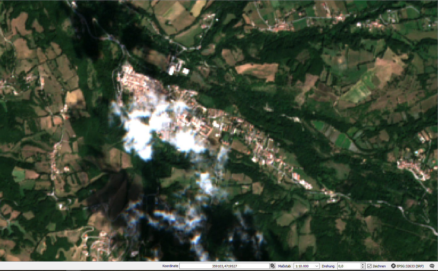
Here is the image taken before the Earthquake.

Note that the resolution of Sentinel-2 images is of 10m. More detailed imageries would have been welcomed for a more precise damage analysis.
Here’s the view just after.
Unfortunately for our analyses, several clouds hide the village at that moment during the day.
We decided anyway to continue our analyses using our formerly described change detection techniques.
Applying a change detection, our final result is the following one.

The centre of the village is highlighted in the blue circle. There have been a lot of damage. The big white areas are the uninvited clouds and the red areas in the South are no other that the shadows of other clouds.
Using the following formula, we were able to determine the number of hectares affected by the damage in the blue cirle.
-- Count the area affected by the damage
SELECT sum(total)/1000 || ' ha' FROM
(SELECT (pvc).VALUE, (pvc).COUNT total
FROM (SELECT ST_ValueCount(rast) As pvc FROM sum_delta_b02_b03_b04 r WHERE ST_Intersects(r.rast, ST_GeomFromText('POLYGON((359769.499 4721124.630, 359711.290 4721016.151, 359520.790 4720889.151, 359412.311 4720957.943, 359465.228 4721317.776, 359803.894 4721196.068, 359769.499 4721124.630))', 32633))) As a
WHERE (pvc).VALUE = 1
ORDER BY (pvc).value) As b;
We get a result of 3.167 ha.
Here a comparison made with WorldView-2 satellite images, with a resolution of 0.46 m.


Cheers,
Daniel
Change detection using Sentinel-2 and PostGIS
August 24th, 2016With its very short revisiting period, Sentinel-2 satellite data make it possible to perform change detection operations of every point on Earth every 5 days at least. In this article, we’re going to apply change detection techniques over the region of Liege, Belgium, between the periods of the 3rd December 2015 and the 11th August 2016, in order to spot changes that may occur during this period.
Here’s how we proceed.
- Data acquisition
- Data format transformation
- Data loading (PostGIS)
- Clipping the data
- Change Dectection formula application
- Results Interpretation
Data acquisition
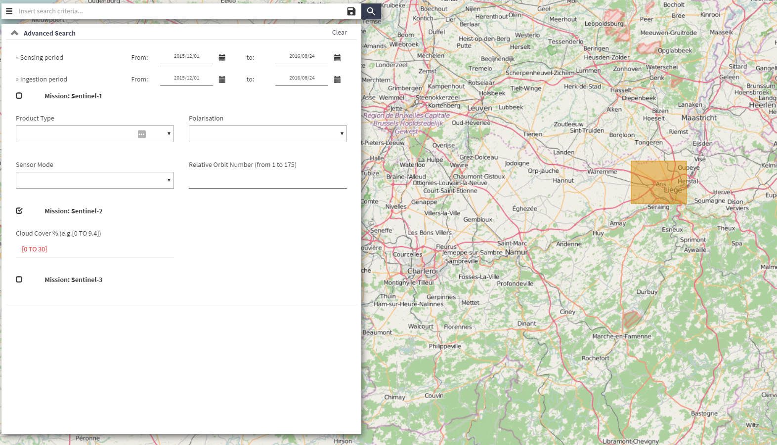
Our area of study this time is the region of Liege, in the Eastern part of Belgium.

Download the Sentinel-2 data by going on the Sentinels Scientific Data Hub webpage. Create an account if you do not have already one. Draw a box in the area of interest and provide information about the wished data. In our example, we’re searching for Sentinel-2 data with cloud percentages of between 0 and 30%. The timestamp is set to be between the 1st of December 2015 and the 24th of August 2016.
Download the following data:
- S2A_OPER_PRD_MSIL1C_PDMC_20151203T172007_R051_V20151203T105818_20151203T105818
- S2A_OPER_PRD_MSIL1C_PDMC_20160811T035114_R008_V20160806T104032_20160806T104026
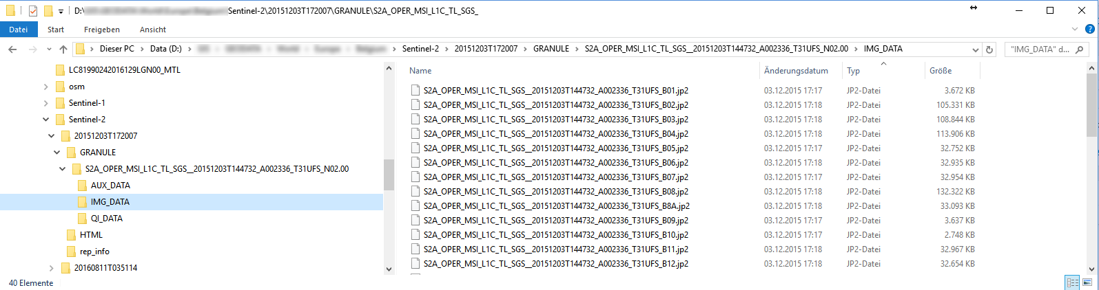
Unzip the data and the structure should look like this.
Data Format Transformation
Our goal is to upload these jp2000 data into our PostGIS database. First, we need to convert these data into the geotiff format using gdal_translate.
d:
cd [...]\Sentinel-2\20151203T172007\GRANULE\S2A_[...]_N02.00\IMG_DATA
gdal_translate.exe -of GTIFF S2A_[...]_B01.jp2 S2A_[...]_B01.tif
gdal_translate.exe -of GTIFF S2A_[...]_B02.jp2 S2A_[...]_B02.tif
gdal_translate.exe -of GTIFF S2A_[...]_B03.jp2 S2A_[...]_B03.tif
gdal_translate.exe -of GTIFF S2A_[...]_B04.jp2 S2A_[...]_B04.tif
[...]
cd D[...]\Sentinel-2\20160811T035114\GRANULE\S2A_[...]_N02.04\IMG_DATA
gdal_translate.exe -of GTIFF S2A_[...]_B01.jp2 S2A_[...]_B01.tif
gdal_translate.exe -of GTIFF S2A_[...]_B02.jp2 S2A_[...]_B02.tif
gdal_translate.exe -of GTIFF S2A_[...]_B03.jp2 S2A_[...]_B03.tif
gdal_translate.exe -of GTIFF S2A_[...]_B04.jp2 S2A_[...]_B04.tif
[...]
Let’s now upload our data into the database.
Data loading (PostGIS)
Create, first, the database.
REM First, change the change the character page to UTF8
chcp 65001
REM Now connect with the postgres credentials
psql -h<ip-address> -Upostgres

-- Change the client_encoding to UTF8 so that it matches the encoding of the Windows Console
set client_encoding to 'UTF8';
-- Change the font of the window to LUCIDA CONSOLE (accents can be seen<ip-address>)

CREATE DATABASE change_detection WITH OWNER themagiscian;
-- Connect to the database as postgres user
psql -h<ip-address> -Upostgres -dchange_detection
CREATE EXTENSION postgis;
-- Enable also the raster capabilities
sudo psql -f /usr/share/postgresql/9.4/contrib/postgis-2.1/rtpostgis.sql -Upostgres -h<ip-address> -dchange_detection
Load the data using the raster2pgsql extension.
REM DECEMBER
raster2pgsql -c -C -s 32631 -f rast -F -I -M -t 100x100 /[...]/S2A_[...]_B01.TIF public.december_b01 | psql -Uthemagiscian -h<ip-address> -dchange_detection
raster2pgsql -d -C -s 32631 -f rast -F -I -M -t 100x100 /[...]/S2A_[...]_B02.TIF public.december_b02 | psql -Uthemagiscian -h<ip-address> -dchange_detection
raster2pgsql -d -C -s 32631 -f rast -F -I -M -t 100x100 /[...]/S2A_[...]_B03.TIF public.december_b03 | psql -Uthemagiscian -h<ip-address> -dchange_detection
raster2pgsql -d -C -s 32631 -f rast -F -I -M -t 100x100 /[...]/S2A_[...]_B04.TIF public.december_b04 | psql -Uthemagiscian -h<ip-address> -dchange_detection
[...]

REM AUGUST
raster2pgsql -c -C -s 32631 -f rast -F -I -M -t 100x100 /[...]/S2A_[...]_B01.TIF public.august_b01 | psql -Uthemagiscian -h<ip-address> -dchange_detection
raster2pgsql -d -C -s 32631 -f rast -F -I -M -t 100x100 /[...]/S2A_[...]_B02.TIF public.august_b02 | psql -Uthemagiscian -h<ip-address> -dchange_detection
raster2pgsql -d -C -s 32631 -f rast -F -I -M -t 100x100 /[...]/S2A_[...]_B03.TIF public.august_b03 | psql -Uthemagiscian -h<ip-address> -dchange_detection
raster2pgsql -d -C -s 32631 -f rast -F -I -M -t 100x100 /[...]/S2A_[...]_B04.TIF public.august_b04 | psql -Uthemagiscian -h<ip-address> -dchange_detection
[...]
For the full list of parameters and their meaning, please refer to this page.
Clipping the data
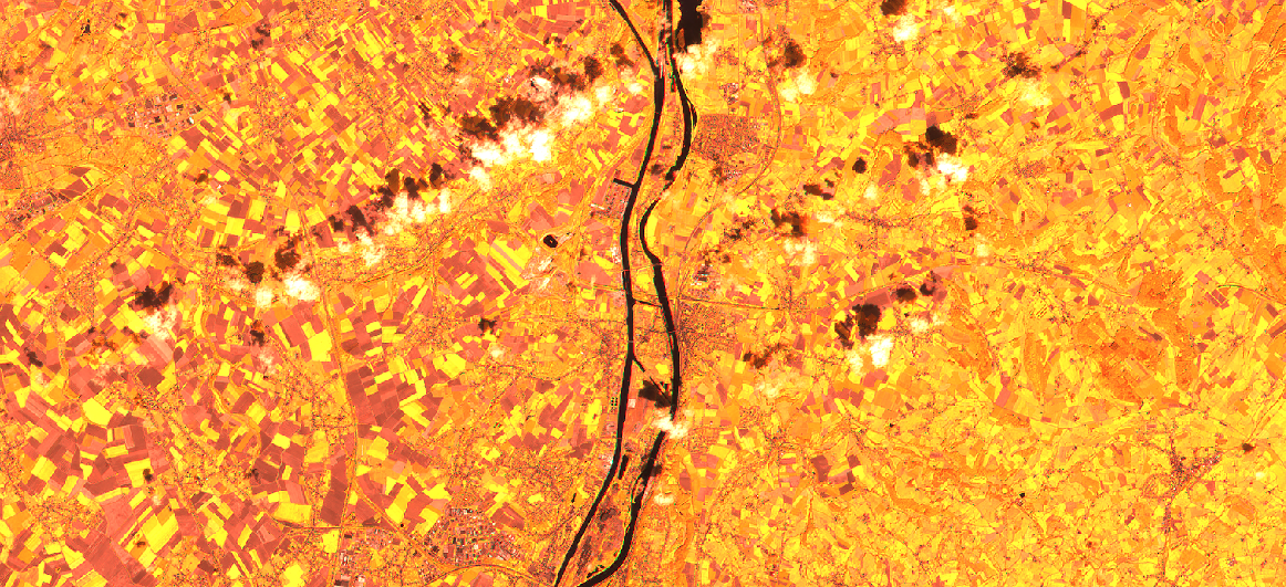
The data we aquired cover a large area. From the dataset of December, we see that a large part of the image is covered with clouds. It doesn’t make sense to perform processing on this very huge part and to waste processing power and time. We focus our attention on the image part that matters and we therefore clip the data on the area of interest.
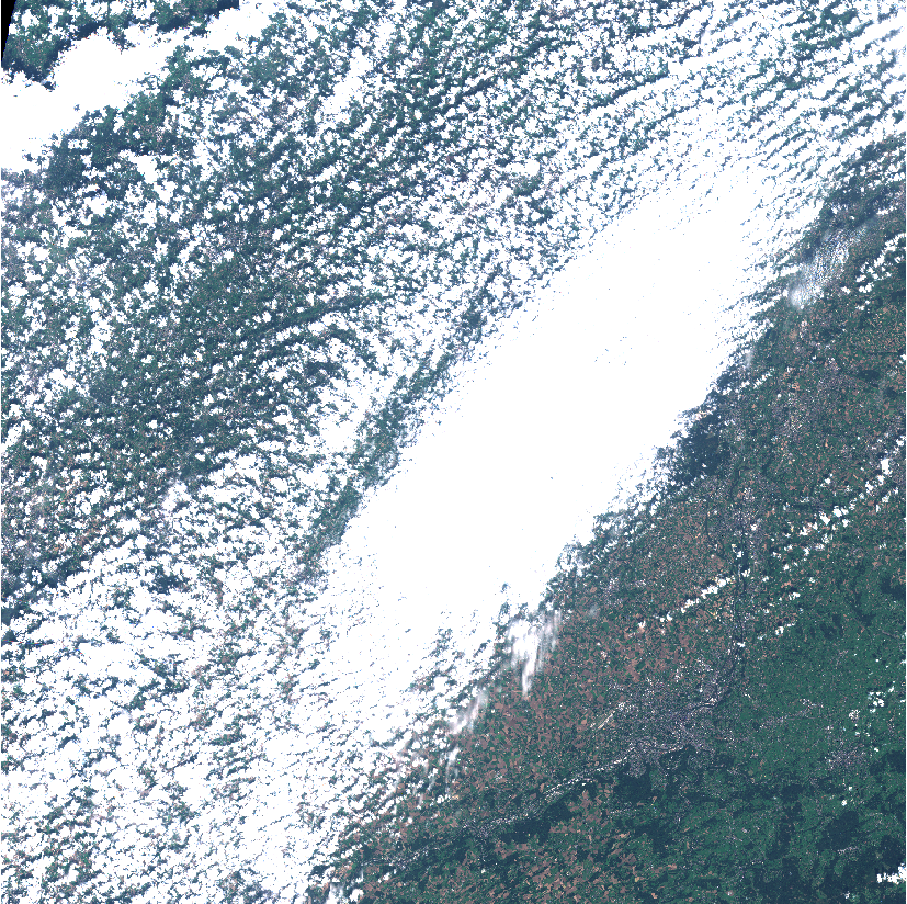
We’re only interested in the South-Eastern part of the image.
DROP TABLE december_b01_clipped;
CREATE TABLE december_b01_clipped AS SELECT * FROM december_b01 r WHERE ST_Intersects(r.rast, ST_GeomFromText('POLYGON((674375.662 5631306.177, 709669.222 5631306.177, 709669.222 5590167.659, 646886.733 5590167.659, 674375.662 5631306.177))', 32631));
DROP TABLE december_b02_clipped;
CREATE TABLE december_b02_clipped AS SELECT * FROM december_b02 r WHERE ST_Intersects(r.rast, ST_GeomFromText('POLYGON((674375.662 5631306.177, 709669.222 5631306.177, 709669.222 5590167.659, 646886.733 5590167.659, 674375.662 5631306.177))', 32631));
DROP TABLE december_b03_clipped;
CREATE TABLE december_b03_clipped AS SELECT * FROM december_b03 r WHERE ST_Intersects(r.rast, ST_GeomFromText('POLYGON((674375.662 5631306.177, 709669.222 5631306.177, 709669.222 5590167.659, 646886.733 5590167.659, 674375.662 5631306.177))', 32631));
DROP TABLE december_b04_clipped;
CREATE TABLE december_b04_clipped AS SELECT * FROM december_b04 r WHERE ST_Intersects(r.rast, ST_GeomFromText('POLYGON((674375.662 5631306.177, 709669.222 5631306.177, 709669.222 5590167.659, 646886.733 5590167.659, 674375.662 5631306.177))', 32631));
[...]

DROP TABLE august_b01_clipped;
CREATE TABLE august_b01_clipped AS SELECT * FROM august_b01 r WHERE ST_Intersects(r.rast, ST_GeomFromText('POLYGON((674375.662 5631306.177, 709669.222 5631306.177, 709669.222 5590167.659, 646886.733 5590167.659, 674375.662 5631306.177))', 32631));
DROP TABLE august_b02_clipped;
CREATE TABLE august_b02_clipped AS SELECT * FROM august_b02 r WHERE ST_Intersects(r.rast, ST_GeomFromText('POLYGON((674375.662 5631306.177, 709669.222 5631306.177, 709669.222 5590167.659, 646886.733 5590167.659, 674375.662 5631306.177))', 32631));
DROP TABLE august_b03_clipped;
CREATE TABLE august_b03_clipped AS SELECT * FROM august_b03 r WHERE ST_Intersects(r.rast, ST_GeomFromText('POLYGON((674375.662 5631306.177, 709669.222 5631306.177, 709669.222 5590167.659, 646886.733 5590167.659, 674375.662 5631306.177))', 32631));
DROP TABLE august_b04_clipped;
CREATE TABLE august_b04_clipped AS SELECT * FROM august_b04 r WHERE ST_Intersects(r.rast, ST_GeomFromText('POLYGON((674375.662 5631306.177, 709669.222 5631306.177, 709669.222 5590167.659, 646886.733 5590167.659, 674375.662 5631306.177))', 32631));
[...]

ALTER TABLE december_b01_clipped ADD CONSTRAINT december_b01_clipped_pk PRIMARY KEY (rid);
ALTER TABLE december_b02_clipped ADD CONSTRAINT december_b02_clipped_pk PRIMARY KEY (rid);
ALTER TABLE december_b03_clipped ADD CONSTRAINT december_b03_clipped_pk PRIMARY KEY (rid);
ALTER TABLE december_b04_clipped ADD CONSTRAINT december_b04_clipped_pk PRIMARY KEY (rid);
[...]

ALTER TABLE august_b01_clipped ADD CONSTRAINT august_b01_clipped_pk PRIMARY KEY (rid);
ALTER TABLE august_b02_clipped ADD CONSTRAINT august_b02_clipped_pk PRIMARY KEY (rid);
ALTER TABLE august_b03_clipped ADD CONSTRAINT august_b03_clipped_pk PRIMARY KEY (rid);
ALTER TABLE august_b04_clipped ADD CONSTRAINT august_b04_clipped_pk PRIMARY KEY (rid);
[...]

SELECT AddRasterConstraints('december_b01_clipped'::name, 'rast'::name);
SELECT AddRasterConstraints('december_b02_clipped'::name, 'rast'::name);
SELECT AddRasterConstraints('december_b03_clipped'::name, 'rast'::name);
SELECT AddRasterConstraints('december_b04_clipped'::name, 'rast'::name);
[...]

SELECT AddRasterConstraints('august_b01_clipped'::name, 'rast'::name);
SELECT AddRasterConstraints('august_b02_clipped'::name, 'rast'::name);
SELECT AddRasterConstraints('august_b03_clipped'::name, 'rast'::name);
SELECT AddRasterConstraints('august_b04_clipped'::name, 'rast'::name);
[...]
Change Detection formula application
In this article, we only focus on “visual” changes. For Sentinel-2 data, the visible bands are the band number 2, 3 and 4 (BGR). Our formula checks the pixels value changes between the imageries of December and August. More precisely, our fomulae is the following.

DROP TABLE delta_aug_dec_b02;
CREATE TABLE delta_aug_dec_b02 AS
SELECT joined.rid, ST_MapAlgebra(arast, 1, brast, 1, 'ROUND([rast1] - [rast2])*([rast1] - [rast2])', '32BF') AS rast FROM (SELECT a.rid, a.rast as arast, b.rast as brast FROM august_b02_clipped a INNER JOIN december_b02_clipped b ON a.rid = b.rid) AS joined;
ALTER TABLE delta_aug_dec_b02 ADD CONSTRAINT delta_aug_dec_b02_pk PRIMARY KEY (rid);
SELECT AddRasterConstraints('delta_aug_dec_b02'::name, 'rast'::name);

DROP TABLE delta_aug_dec_b03;
CREATE TABLE delta_aug_dec_b03 AS
SELECT joined.rid, ST_MapAlgebra(arast, 1, brast, 1, 'ROUND([rast1] - [rast2])*([rast1] - [rast2])', '32BF') AS rast FROM (SELECT a.rid, a.rast as arast, b.rast as brast FROM august_b03_clipped a INNER JOIN december_b03_clipped b ON a.rid = b.rid) AS joined;
ALTER TABLE delta_aug_dec_b03 ADD CONSTRAINT delta_aug_dec_b03_pk PRIMARY KEY (rid);
SELECT AddRasterConstraints('delta_aug_dec_b03'::name, 'rast'::name);

DROP TABLE delta_aug_dec_b04;
CREATE TABLE delta_aug_dec_b04 AS
SELECT joined.rid, ST_MapAlgebra(arast, 1, brast, 1, 'ROUND([rast1] - [rast2])*([rast1] - [rast2])', '32BF') AS rast FROM (SELECT a.rid, a.rast as arast, b.rast as brast FROM august_b04_clipped a INNER JOIN december_b04_clipped b ON a.rid = b.rid) AS joined;
ALTER TABLE delta_aug_dec_b04 ADD CONSTRAINT delta_aug_dec_b04_pk PRIMARY KEY (rid);
SELECT AddRasterConstraints('delta_aug_dec_b04'::name, 'rast'::name);

-- Two-step formula as ST_MapAlgebra only takes two raster documents
DROP TABLE sum_delta_aug_dec_b02_b03;
CREATE TABLE sum_delta_aug_dec_b02_b03 AS
SELECT joined.rid, ST_MapAlgebra(arast, 1, brast, 1, 'ROUND([rast1] + [rast2])', '32BF') AS rast FROM (SELECT a.rid, a.rast as arast, b.rast as brast FROM delta_aug_dec_b02 a INNER JOIN delta_aug_dec_b03 b ON a.rid = b.rid) AS joined;
ALTER TABLE sum_delta_aug_dec_b02_b03 ADD CONSTRAINT sum_delta_aug_dec_b02_b03_pk PRIMARY KEY (rid);

DROP TABLE sum_delta_aug_dec_b02_b03_b04;
CREATE TABLE sum_delta_aug_dec_b02_b03_b04 AS
SELECT joined.rid, ST_MapAlgebra(arast, 1, brast, 1, 'ROUND(SQRT([rast1] + [rast2]))', '32BF') AS rast FROM (SELECT a.rid, a.rast as arast, b.rast as brast FROM sum_delta_aug_dec_b02_b03 a INNER JOIN delta_aug_dec_b04 b ON a.rid = b.rid) AS joined;
ALTER TABLE sum_delta_aug_dec_b02_b03_b04 ADD CONSTRAINT sum_delta_aug_dec_b02_b03_b04_pk PRIMARY KEY (rid);

-- Convert the raster document into a binary mask
UPDATE sum_delta_aug_dec_b02_b03_b04 SET rast = ST_Reclass(rast, '0-1500:0, 1500-55635:1', '2BUI');
Notice that the values chosen for the the final classification has been defined by try and error in QGIS.
Results interpretation
The final document is the following. Each red area represent places where a significant change is visible.
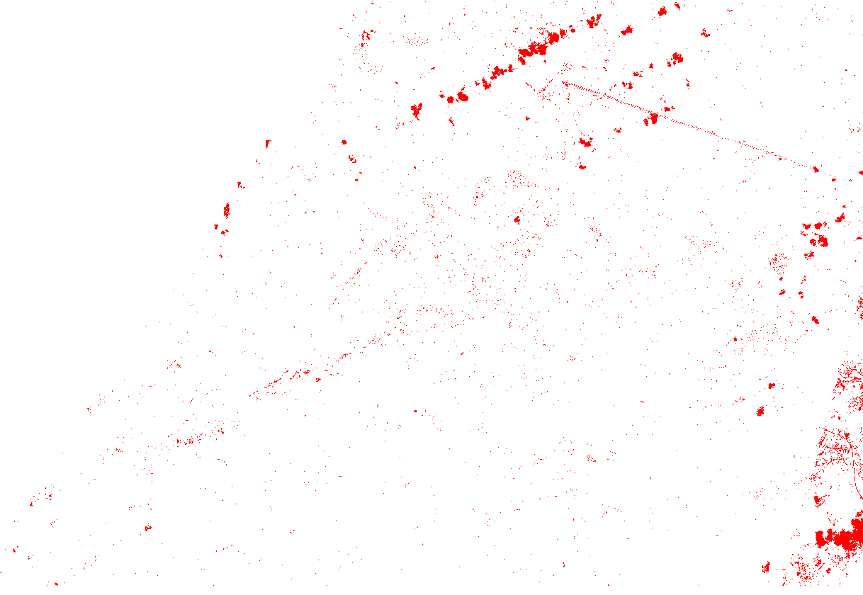
Most spots are due to the clouds that are present on the August imagery. We could could remove these “false results” by detecting the clouds using band combination 568. Clouds are the only feature in bright white.
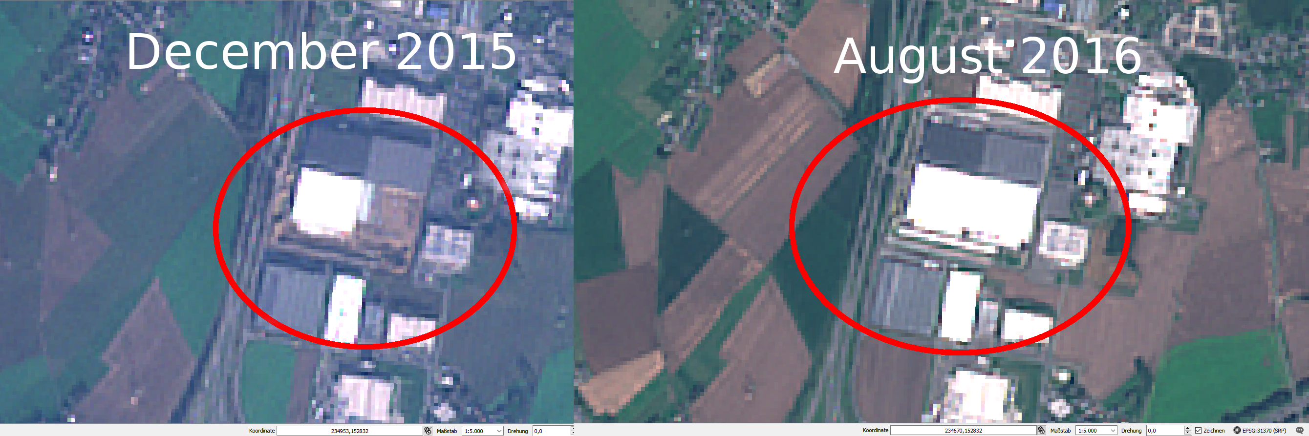
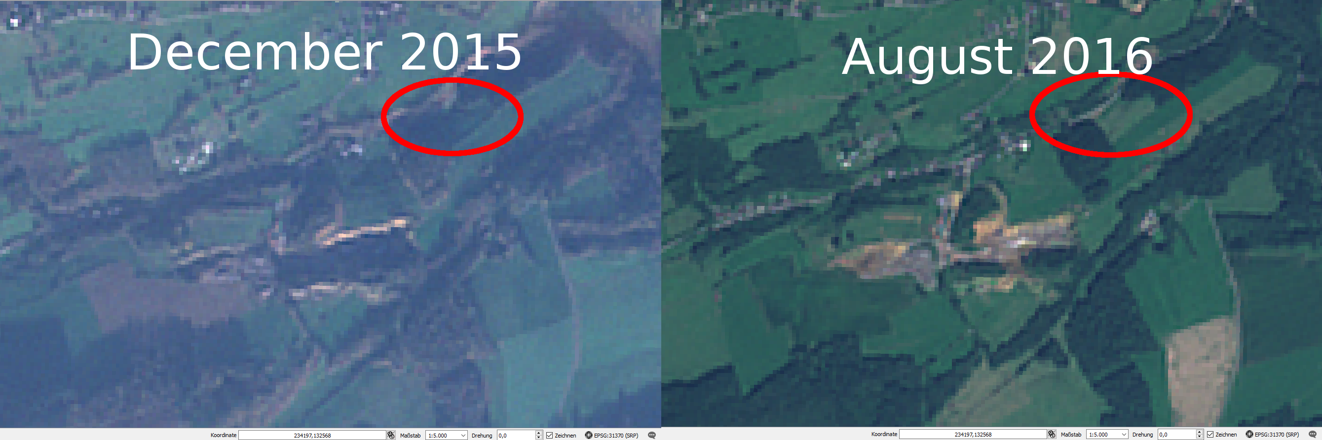
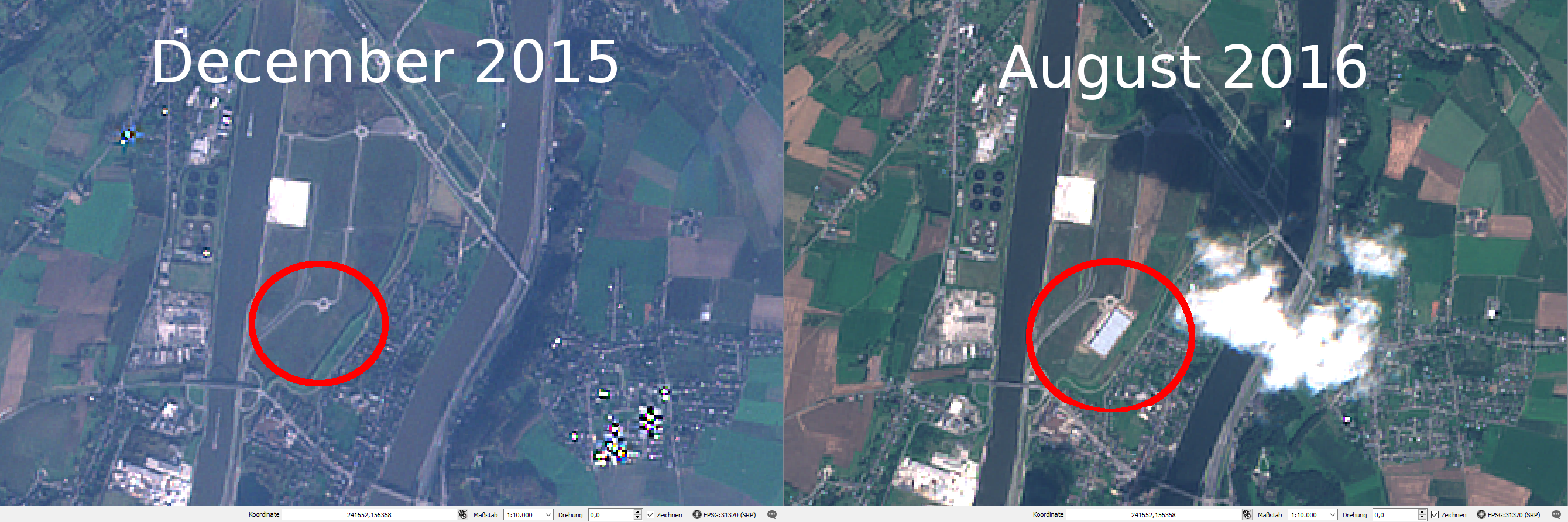
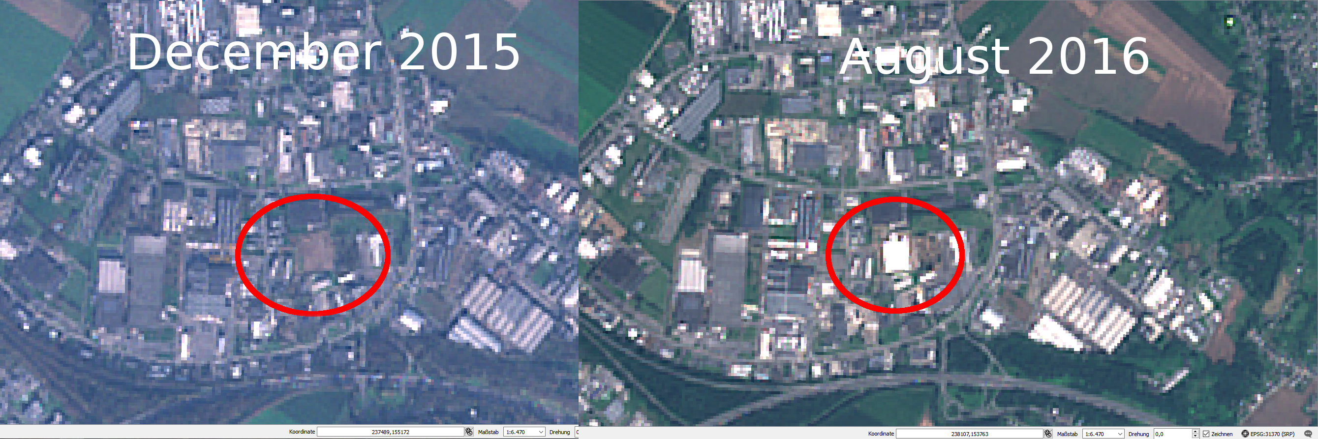
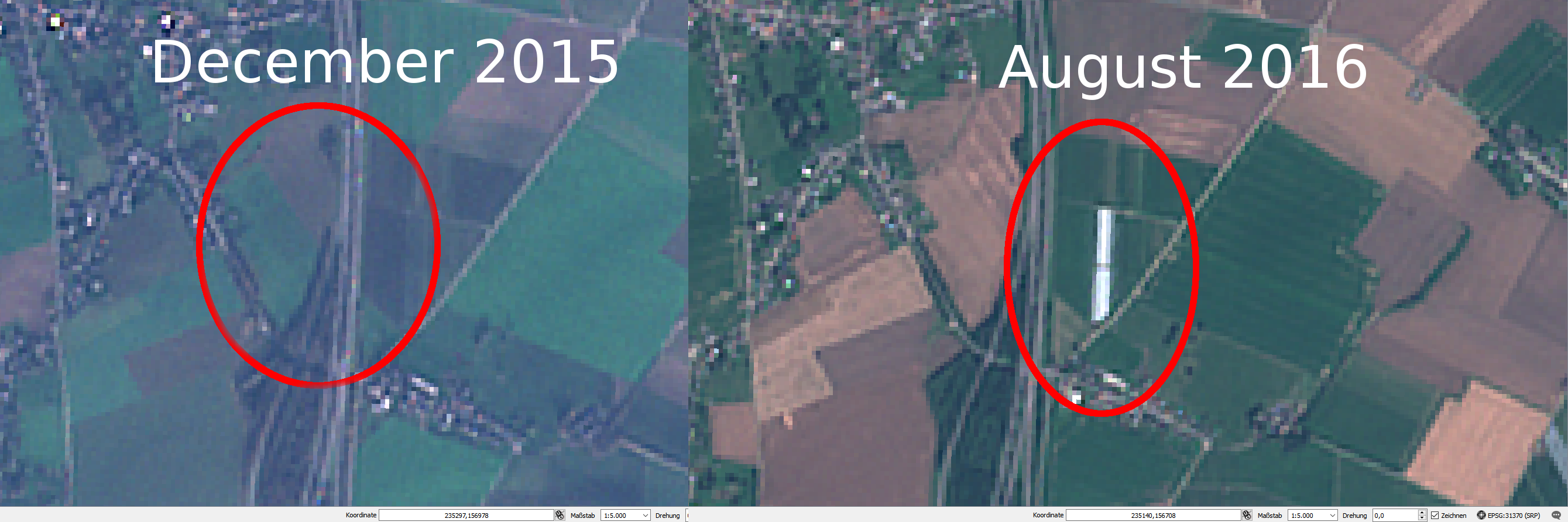
By zooming on the red spots, let’s discover what has changed.
We found mostly places where new buildings arose from the ground.
Here, a new building were built in the Business Park Les Hauts Sarts
A small parcel with trees having been cut
A new building appears at the site where the Trilogiport is built in the Northern Part of Liege.
Another building built in the Business Park Les Hauts Sarts
Our last example is about an agricultural building
Conclusions
With the available Sentinel-2 data and our remote sensing techniques, we were able to set up a semi-automatic way of applying a change detection processing. Our final document, which is the mask, gives us an insights about spots where things changed over time. Conlusions and analytics must always be performed by a human operator in order to weight more efficiently what did change.
Our data were those of December and August. By retrieving Sentinel-2 images in between this period we would have a finer temporal approach about when these things changed.
The techniques we applied can still be enhanced and we could run an intermediate “cloud-detection” algorithm in order to remove some disturbances.
Why so many -ange places in Belgium near Luxembourg?
August 14th, 2016Belgium’s petrol station!
The South of Belgium is a beautiful place covered mostly with the region Ardennes – a forested landscape where Belgian used to go out at the weekends to relax. On their road to the South, Belgians also like doing a small stop in the neighbouring country Luxembourg! Petrol, alcool and cigarettes is far much cheaper in Luxembourg!
What characterizes also the very Southern part of the country as well as villages in Luxembourg especially are the village names ending with “-ange”, like Martelange, Grumelange, Hollange, Aubange, etc.
Where do the “-ange” come from?
Belgium and the cultural influences
Belgium is a very small country in the Western part of Europe. It lies between The Netherlands, Germany, Luxembourg and France. Despite being so small – around 30 528 km²/11 787 sq mi or the size of Massachusetts – it has a marvelous cultural landscape and has successively received, along history, Celtic, Latin, Germanic, Saxon, Dutch, French and German influences.
These influences have shaped the toponyms (place names) and it is still possible today to retrace the origins of most names of villages and towns. The origins are often seen in the suffixes and this leads us to think that all places with similar suffixes have the same origin. This is often true but not always.
Most of the place names are nowadays very strongly influenced by the language region they are located in. Belgium has 3 national languages: Flemish (spoken in the Northern part of Belgium), French (spoken in the Southern part), and German (spoken in the Eastern part). Brussels is considered being bilingual (Flemish and French) but most of the inhabitants speak French.
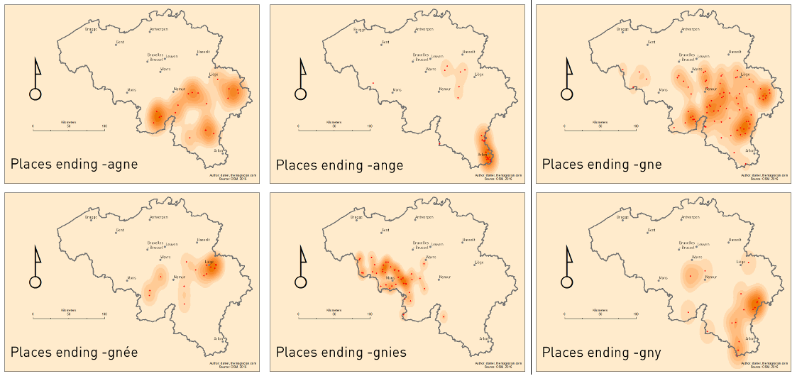
In this articles, we focus on villages and towns ending with –ange, but also with the derivatives –agne, –gne, –gnée, –gnies and –gny.
I want to work for your GIS Missions
August 13th, 2016Ready for your GIS missions!

It is a great pleasure to announce that themagiscian.com is now open for YOUR gis missions! We have now a juridic existence in Belgium and working with a valid VAT number. We’re available for your gis missions abroad a well!
Let’s CREATE GREAT adventures!

A Hooded Vulture Wildlife study using Movebank, PostGIS, QGIS and KML
August 5th, 2016Movebank.org is fabulous website that centralizes GPS data of tracked animals. Hosted by the Max Planck Institute for Ornithology, the platform data are accessible to researchers from all over the world to study animal movements ranging from cats and dogs to hooded vulture.
We decide to download data related to a Hooded Vulture in the Kruger National Park, South Africa, to illustrate how one could get most of this data. Simply go the Movebank Website on the map and search for Hooded Vulture in the Search Box. Then download the data in csv format.

Notice that no height or Z value information is available in the csv. What we’re now interested to extract the positions and the timestamps. Our objective is to learn a lot about the movements of the animals in terms of hunting ground, behavior, and seeing the animated movements in Google Earth. We’re at ease using a database to perform any query we want. So we’re using PostGIS.
Here are the steps for our studies.
- Create the PostGIS database
- Create the table and import the csv data
- Create the geometry field
- Create the Hooded Vulture paths (connect points by lines)
- Get Basic Statistics and create the map in QGIS
- Create the KML file
- Visualize the animation in Google Earth
Create the database
First connect to the database (open a command line window): psql -h<ip-address> -Upostgres
Create the database:
CREATE DATABASE animal_tracking WITH OWNER themagiscian;
Connect to the database with an admin as we want to enable the PostGIS cartridge.
psql -h<ip-address> -Upostgres -danimal_tracking
CREATE EXTENSION postgis;
You can now connect with your normal user. Note that the first line set the prompt window in UTF8 mode. We do the same for the psql interface once connected.
chcp 65001
psql -h192.168.1.87 -Uthemagiscian -danimal_tracking
SET client_encoding to 'UTF8'
Create the table and import the csv data
We’re now ready to import the data coming from the csv file.
First, create the table that will welcome the data. We got the column names from the csv file we opened in Excel. We quoted all the names because they are whether reserved keyword or they contain non-acceptable chars such as semicolon, colon, etc.
CREATE TABLE hooded_vulture_positions (
 "event-id" numeric(10),
 "visible" boolean,
 "timestamp" timestamp,
 "location-long" double precision,
 "location-lat" double precision,
 "external-temperature" double precision,
 "gps:satellite-count" numeric,
 "gps-time-to-fix" double precision,
 "ground-speed" double precision,
 "gt:activity-count" numeric,
 "gt:sys-week" numeric,
 "gt:tx-count" numeric,
 "heading" double precision,
 "height-above-ellipsoid" double precision,
 "height-raw" varchar(7),
 "location-error-text" varchar(50),
 "manually-marked-outlier" double precision,
 "tag-voltage" double precision,
 "vertical-error-numerical" double precision,
 "sensor-type" varchar(22),
 "individual-taxon-canonical-name" varchar(20),
 "tag-local-identifier" varchar(6),
 "individual-local-identifier" varchar(20),
 "study-name" varchar(21)

);
Load the table.
\copy hooded_vulture_positions FROM '/<path_to_the_file>/Hooded Vulture Africa.csv' HEADER DELIMITER ',' CSV;
Create the geometry field
The csv data file contains longitudes and latitudes. We need to create a specific geom field if we want to perform geographic processing in order to analyse the movement and if we want to see some results on a map in QGIS.
ALTER TABLE hooded_vulture_positions ADD COLUMN geom geometry;
UPDATE hooded_vulture_positions SET geom = ST_SetSRID(ST_MakePoint("location-long", "location-lat"), 4326);
SELECT UpdateGeometrySRID('hooded_vulture_positions','geom',4326);
CREATE INDEX hooded_vulture_positions_gix ON hooded_vulture_positions USING GIST (geom);
VACUUM ANALYZE hooded_vulture_positions;
Create the Hooded Vulture paths (connect points by lines)
The next step is to connect the consecutive points with each other.
Create first the table.
DROP TABLE hooded_vulture_lines;
CREATE TABLE hooded_vulture_lines AS SELECT "event-id" AS "from-event-id", "event-id" AS "to-event-id",
"timestamp" AS "from-timestamp", "timestamp" AS "to-timestamp", geom FROM hooded_vulture_positions WITH NO DATA;
The function used to connect points is ST_MakeLine. The thing is that we first classify the points based on the timestamp and then we connect each consecutive point. The best way to performit is to loop through the table. We do that using the following PL/SQL script. Notice how we focus on the tag-local-identifier 139251. In fact, the csv file we downloaded contains several individuals and we want to focus only on one.
CREATE OR REPLACE FUNCTION create_lines() RETURNS void AS
$BODY$
DECLARE
 r hooded_vulture_positions%rowtype;
 old_eventidfrom numeric;
 old_timestamp timestamp;
 old_geom geometry;
BEGIN
 FOR r IN SELECT * FROM hooded_vulture_positions WHERE "tag-local-identifier" = '139251' ORDER BY "timestamp" ASC
 LOOP
 INSERT INTO hooded_vulture_lines VALUES (old_eventidfrom, r."event-id", old_timestamp, r."timestamp", ST_MakeLine(old_geom, r.geom));
 old_eventidfrom := r."event-id";
 old_timestamp := r."timestamp";
 old_geom := r.geom;
 END LOOP;
END
$BODY$
LANGUAGE 'plpgsql' ;
Execute the function.
SELECT create_lines();
A clean job involves setting the correct SRS and indexing the data.
SELECT UpdateGeometrySRID('hooded_vulture_lines','geom',4326);
CREATE INDEX hooded_vulture_lines_gix ON hooded_vulture_lines USING GIST (geom);
For information, we create a new field with the length of each segment.
ALTER TABLE hooded_vulture_lines ADD COLUMN distance double precision;
UPDATE hooded_vulture_lines SET distance = ST_Length(geom::geography)/1000;
Get Basic Statistics
All the previous jobs were done to make it possible to perform statistics on the data and to make the map using QGIS.
How many positions do we have?
SELECT count(*) from hooded_vulture_positions WHERE "tag-local-identifier" = '139251';
 count
-------
 9680
In which time interval?
SELECT min("timestamp") as "start", max("timestamp") as "finish" FROM hooded_vulture_positions WHERE "tag-local-identifier" = '139251';
 start | finish
---------------------+---------------------
 2014-12-14 03:00:00 | 2016-08-02 03:00:00
What is the total distance covered during the study time and based on the GPS data?
SELECT sum(ST_Length(geom::geography))/1000 || ' km' as TOTAL_LENGTH FROM hooded_vulture_lines;
 total_length
---------------------
 26264.8193016478 km
What about the busiest days? (lengths are in km)
SELECT EXTRACT(YEAR FROM "from-timestamp") || '/' || LPAD(EXTRACT(MONTH FROM "from-timestamp")::text, 2, '0') || '/' || LPAD(EXTRACT(DAY FROM "from-timestamp")::text, 2, '0') "Date",
 sum(ST_Length(geom::geography))/1000::double precision as total_length FROM hooded_vulture_lines GROUP BY EXTRACT(YEAR FROM "from-timestamp"), EXTRACT(MONTH FROM "from-timestamp"), EXTRACT(DAY FROM "
from-timestamp") ORDER BY total_length desc LIMIT 10;
 Date | total_length
------------+------------------
 |
 2015/06/05 | 177.357438408111
 2015/02/26 | 174.974560854037
 2015/02/18 | 173.766023783359
 2015/03/10 | 162.334720926385
 2015/05/21 | 161.941723565214
 2015/05/03 | 155.456692232334
 2015/10/07 | 150.336621420365
 2015/03/13 | 146.837049519552
 2015/05/10 | 145.162814856346
These results are not surprising as Hooded Vultures can travel as far as 150km a day to find food.
And finallly, we want to know the extreme points: Nothernmost, Southernmost, Easternmost and Westernmost point as well as the centroid of the point cloud. We store these results in a separate table.
-- Northern most point
DROP TABLE hooded_vulture_spatial_statistics;
CREATE TABLE hooded_vulture_spatial_statistics AS SELECT "event-id" as eventid, 'Northernmost point'::varchar(30) as description, "timestamp", ST_Y(geom)::varchar(10) as coordinate, geom FROM hooded_vulture_positions WHERE "tag-local-identifier" = '139251' AND ST_Y(geom) = (SELECT max(ST_Y(geom)) FROM hooded_vulture_positions WHERE "tag-local-identifier" = '139251') LIMIT 1;

-- Sourthernmost point
INSERT INTO hooded_vulture_spatial_statistics SELECT "event-id" as eventid, 'Sourthernmost point'::varchar(30) as description, "timestamp", ST_Y(geom)::varchar(10) as coordinate, geom FROM hooded_vulture_positions WHERE "tag-local-identifier" = '139251' AND ST_Y(geom) = (SELECT min(ST_Y(geom)) FROM hooded_vulture_positions WHERE "tag-local-identifier" = '139251') LIMIT 1;

-- Easternmost point
INSERT INTO hooded_vulture_spatial_statistics SELECT "event-id" as eventid, 'Easternmost point'::varchar(30) as description, "timestamp", ST_X(geom)::varchar(10) as coordinate, geom FROM hooded_vulture_positions WHERE "tag-local-identifier" = '139251' AND ST_X(geom) = (SELECT max(ST_X(geom)) FROM hooded_vulture_positions WHERE "tag-local-identifier" = '139251') LIMIT 1;

-- Westernmost point
INSERT INTO hooded_vulture_spatial_statistics SELECT "event-id" as eventid, 'Westernmost point'::varchar(30) as description, "timestamp", ST_X(geom)::varchar(10) as coordinate, geom FROM hooded_vulture_positions WHERE "tag-local-identifier" = '139251' AND ST_X(geom) = (SELECT min(ST_X(geom)) FROM hooded_vulture_positions WHERE "tag-local-identifier" = '139251') LIMIT 1;

-- Center of gravity of the positions
INSERT INTO hooded_vulture_spatial_statistics SELECT '9999' as eventid, 'Centroid' as description, '2016-08-04 00:00:00.00', '', ST_Centroid(ST_Multi(ST_UNION(geom))) geom FROM hooded_vulture_positions WHERE "tag-local-identifier" = '139251';

SELECT UpdateGeometrySRID('hooded_vulture_spatial_statistics','geom',4326);
CREATE INDEX hooded_vulture_spatial_statistics_gix ON hooded_vulture_spatial_statistics USING GIST (geom);
What we can do with all these analysis is to put them on the map (using QGIS).
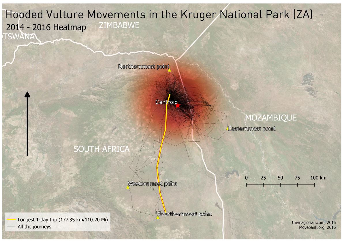
The hooded vulture we’re tracking stays more or less in the same area all the time (end 2014 to mid-2016). The crowdest area is roughly an area of 40km in length and 25km in width with direction NW-SE, except for some longer journeys to the extreme points.
Create the KML file
Up to now we were focused on statistics and situational facts. What about creating an animation in Google Earth and study the behavior of the hooded vulture?
There are several ways of getting a KML file from Movebank.org. The first being to download directly the data in KML format (instead of the CSV as we did). The ogr2ogr utility can extract PostGIS data and convert them into a KML file. But the problem with these solutions is that they do not include the <TimeStamp><when> tags which are necessary to see animations in GE. Working with these files to get them in shape is not an easy matter so we kept the simplest solution: creating our tags directly from an SQL query. It looks like this.
SELECT '<Placemark><TimeStamp><when>' || EXTRACT(YEAR FROM "timestamp") || '-' || LPAD(EXTRACT(MONTH FROM "timestamp")::text, 2, '0')
|| '-' || LPAD(EXTRACT(DAY FROM "timestamp")::text, 2, '0') || 'T' || LPAD(EXTRACT(HOUR FROM "timestamp")::text, 2, '0') || ':' ||
LPAD(EXTRACT(MINUTE FROM "timestamp")::text, 2, '0') || ':' || LPAD(EXTRACT(SECOND FROM "timestamp")::text, 2, '0') || 'Z' ||
'</when></TimeStamp><styleUrl>#hooded_vulture-icon</styleUrl><Point><gx:altitudeMode>relativeToGround</gx:altitudeMode><coordinates>'
|| ST_X(geom) || ',' || ST_Y(geom) || ',30</coordinates></Point></Placemark>' FROM hooded_vulture_positions
WHERE "tag-local-identifier" = '139251' ORDER BY "timestamp" \g hooded_vulture_za_path.kml
We include in the response the needed tags and we format the date and time in a by GE readable format. Notice how we add the Z coordinate to 30 in order to have an altitude value. To not forget are to add the leading zeros in the month and day number (using the LPAD). the \g indicates we’re storing the result in the hooded_vulture_za_path.kml file.
Our KML is not ready to be processed by Google Earth yet. We need to add the headers and the footers.
Paste this into the file at the beginning.
<?xml version="1.0" encoding="UTF-8"?>
<kml xmlns="http://earth.google.com/kml/2.2" xmlns:gx="http://www.google.com/kml/ext/2.2">
 <Document>
 <name>Hooded Vulture Life</name>
 <Style id="hooded_vulture-icon">
 <IconStyle>
 <Icon>
 <href>hooded_vulture_icon.png</href>
 </Icon>
 <hotSpot x="0" y=".5" xunits="fraction" yunits="fraction"/>
 </IconStyle>
 </Style>
 <Style id="check-hide-children">
 <ListStyle>
 <listItemType>checkHideChildren</listItemType>
 </ListStyle>
 </Style>
 <styleUrl>#check-hide-children</styleUrl>
Notice we use a custom symbology: a hooded vulture clipart name hooded_vulture-icon with the path specified in the href. Also use the checkHideChildren value for avoiding having all the 9680 elements listed in he legend of GE.
Paste the footer part in the file and save.
 </Document>
</kml>
Visualize the animation in Google Earth
If the KML is well formed, Google Earth should directly open the animation pane.
Adjust the options (reading speed, time interval, etc.) and enjoy the animation!
This video was created with the Movie Maker feature in Google Earth.
Analyses. What we can see is that the bird is flying almost every day over the valley of the Shingwedzi River. Most of his food can be found in this area assumably. Also interesting, the vulture stays one day West of the study area, and one day East as it would alternate his sleeping place. The distance between these points is approximately 50 km.
Conclusion
This article shows us how to exploit data coming for the valuable Movebank.org website. People are sharing GPS data about their animal friends and getting the most out of the data teaches us a lot. A tremendous amount of statistics can be done and making a Google Earth animation shows us its movement behavior.
All of this is possible using ETL techniques and handling tools such as PostGIS, QGIS and Google Earth.
Cheers,
Daniel
Wildland Fire study with Landsat 7 and PostGIS
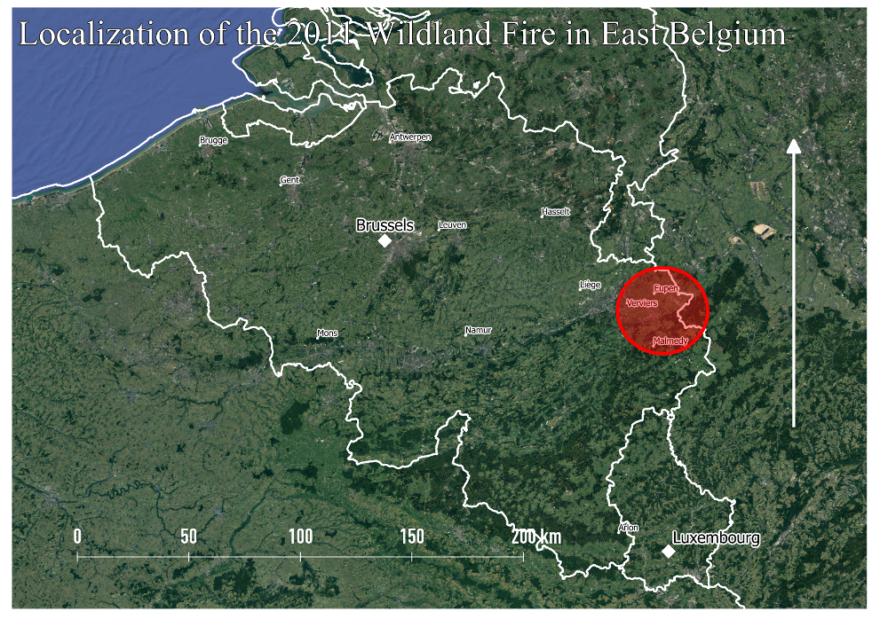
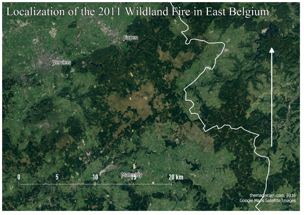
July 30th, 2016Wildland fires commonly occur during the hot and dry seasons. More tempered climates can however also be affected. We are studying the extent of the last major wildland fire that occur the 25 and 26 of April 2011 in East Belgium using Landsat 7 L1 imageries. 1300 ha was burnt during this event that lasted a couple of weeks. Let’s analyse the consequences using remote sensing techniques 🙂
Our study area in the High Fens.
And here a look on the field.
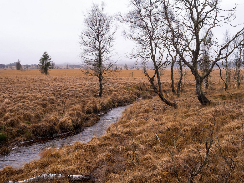
As you can see, in Belgian’s high altitudes (over 600m (2000 ft) above sea level), the landscape is a type of grassy wetland with sparsely densed trees. That’s why we’re talking about wildland fire instead of “forest fire” in this article.
Our first step is to get a sample data of the region taken BEFORE the wildland fire and to compare it with data AFTER.
Crime Data analyses (Tulsa, OK)
July 22nd, 2016Open Crime data are very powerful for predictive crime analyses. Most Police units make use of historical data and GIS to analyze crime patterns and trends. The conclusion drawn from these analyses are used to better place officers more efficiently on the field, for example.
We think it is very interesting to show how historical crime data can be used to analyse crime patterns in space and time, and to present the results to the local authorities. We found the very intersting Open Data Portal of the city of Tulsa, OK, for our analyses. The city provides crime data in Shapefile for the period 2010 – 2014.
See how the crimes spread accross the city for the study period. Notice already some crime hotspots!
Let’s play around with these data and do deeper analysis!
Personal Challenge: Run a Marathon! … or 20km
June 1st, 2016Most “X things to do before you die” lists or articles talking about personal challenges contain “Run a marathon” at the top. I took this challenge just halfway (or a little less) by running the 20km of Brussels.
I do like practicing sports and I try to do 2-3 sessions of running a week. I do it mostly for keeping in shape as I do not run for beating the clock or achieve performances. Being used to run from 5 to 10 km per session, these 20 km seemed to be very challenging to me!
Gaia, the organisation I support for 5 years now, let me know me about this race in one of their newsletters and I immediately jumped in for them! I ran for them and I thought it could get me out of the routine runnings I try to do several times a week.
The key for me was the personal challenge! I guess we should all set personal challenges like these to keep motivated to get up each morning!
What are/were yours?
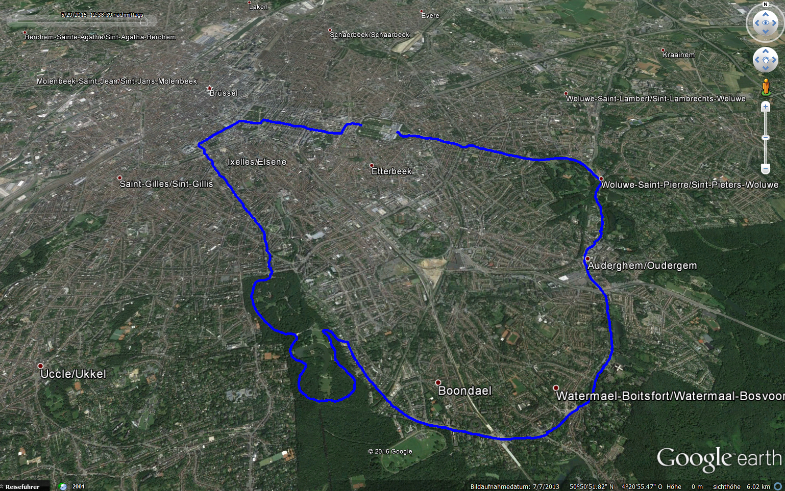
By the way, I did the 20km in 02h06! You can have a look at my performances hereunder by downloading the kml or GPX of the track.
Always been fascinated by the level of detail in Google Earth …
Car navigation: Wrong expected arrival times!
May 22nd, 2016Car navigation systems can sometimes provide VERY erronous information. I did recently need to go by car in another part of the city of Brussels, Belgium. In the absence of public transportation, due to the terrorist attacks that occur just a few days before, I had to take the car for just around 6 kilometers. It was 17:20 and the arrival time was expected to be at 17:35. I was however caught in heavy traffic jams (oh surprise!). I finally did arrive at … 17:52. In normal times, traffic jams are very common and as public transportation were down, the streets were even more loaded than in normal times.
Holy placenames in Belgium
May 9th, 2016Placenames in Belgium and the cultural influences
Belgium is a very small country in the Western part of Europe. It lies between The Netherlands, Germany, Luxembourg and France. Despite being so small – around 30 528 km²/11 787 sq mi or the size of Massachusetts – it has a marvelous cultural landscape and has successively received, along history, Celtic, Latin, Germanic, Saxon, Dutch, French and German influences.
These influences have shaped the toponyms (placenames) and it is still possible today to retrace the origins of most names of villages and towns. The origins are often seen in the suffixes and this leads us to think that all places with similar suffixes have the same origin. This is often true but not always.
Nowadays, most of the place names very strongly influenced by the language region they are located in. Belgium has 3 national languages: Flemish (spoken in the Northern part of Belgium), French (spoken in the Southern part), and German (spoken in the Eastern part). Brussels is considered being bilingual (Flemish and French) but most of the inhabitants speak French.
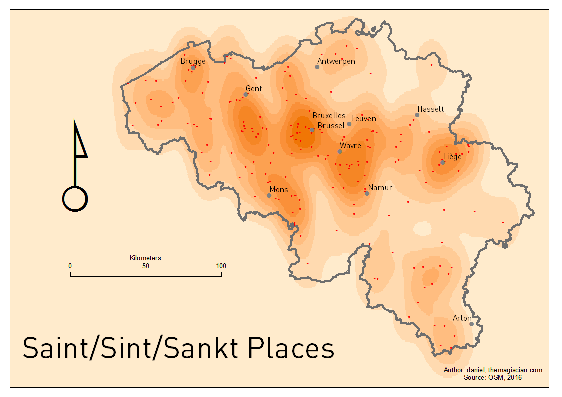
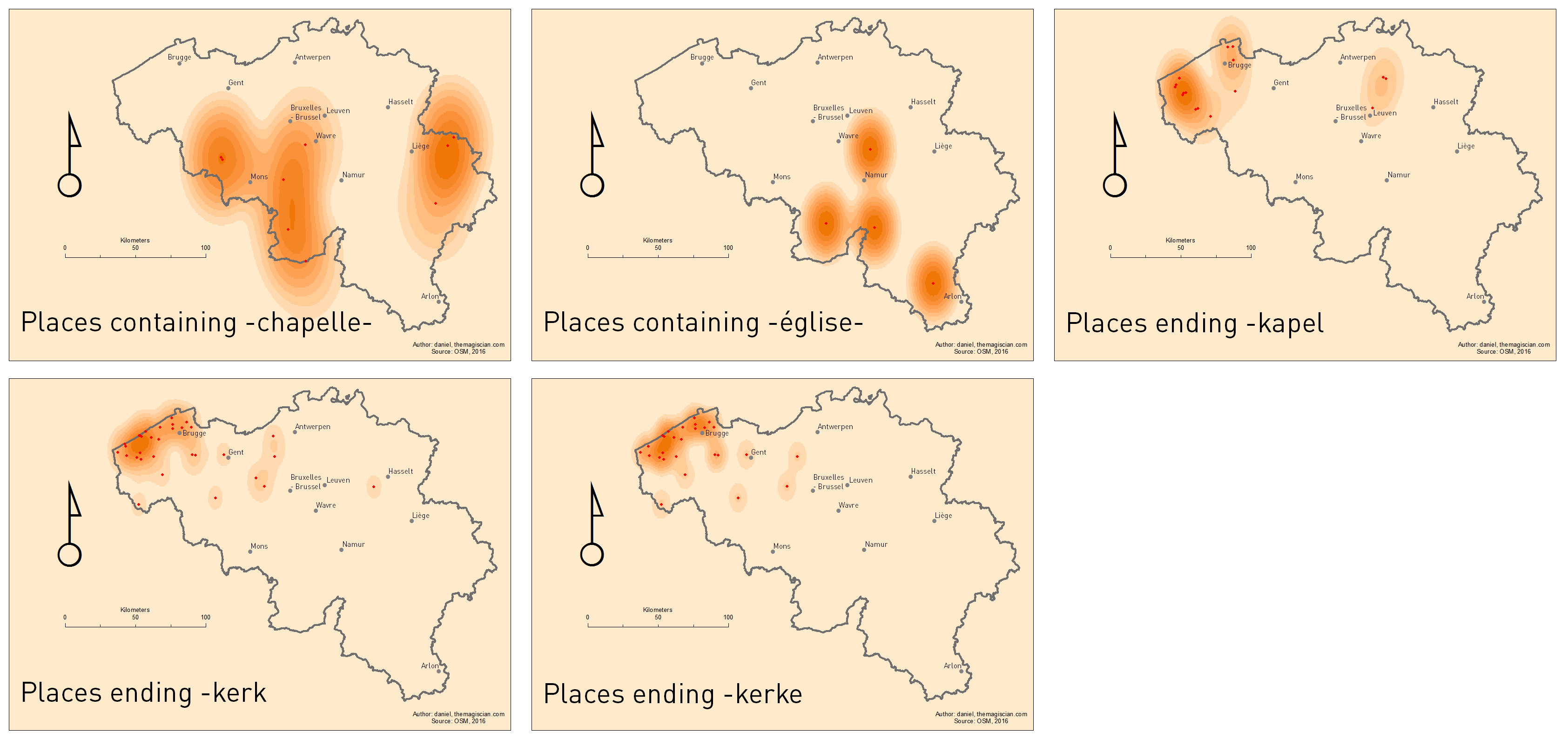
In this articles, we focus on villages and towns containing the sacred word “Saint” (and Dutch and German variation Sint and Sankt), but also other holy places containing holy words such as “Chapelle” (chapel in French), “Eglise” (church in French), “Kapel” (chapel in Flemish), “Kerk” (church in Flemish) and the West Flemish derivative “Kerke“.
Each dot represents a place.