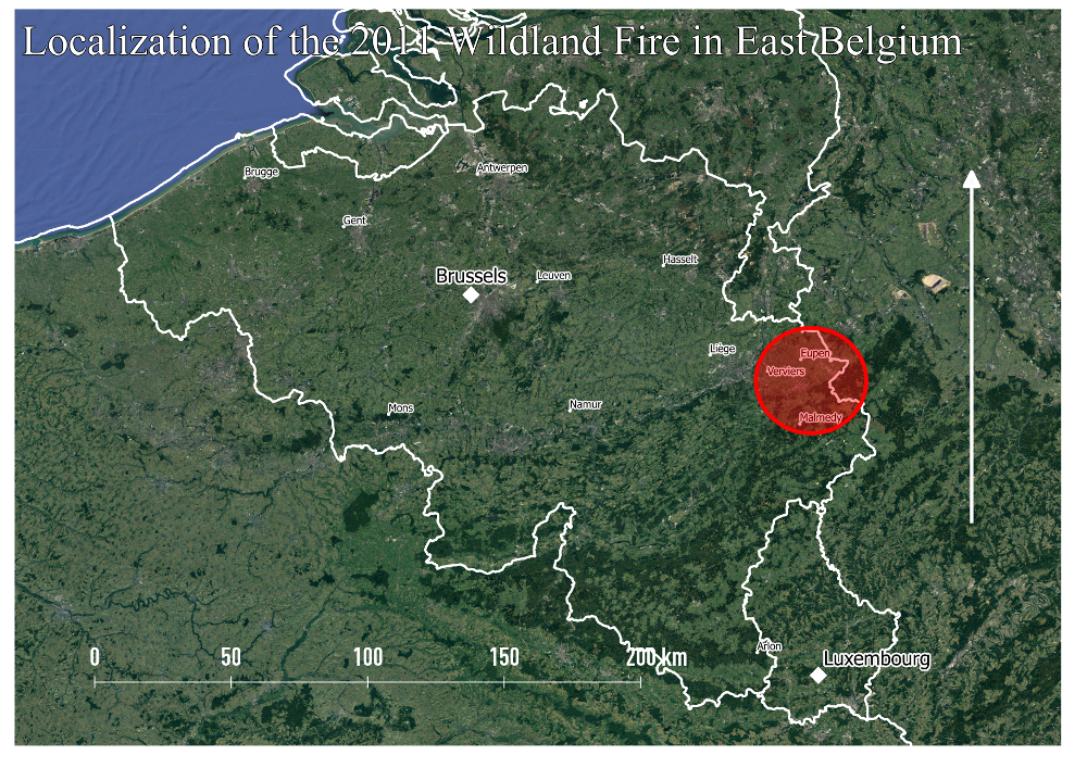
Wildland fires commonly occur during the hot and dry seasons. More tempered climates can however also be affected. We are studying the extent of the last major wildland fire that occur the 25 and 26 of April 2011 in East Belgium using Landsat 7 L1 imageries. 1300 ha was burnt during this event that lasted a couple of weeks. Let’s analyse the consequences using remote sensing techniques 🙂
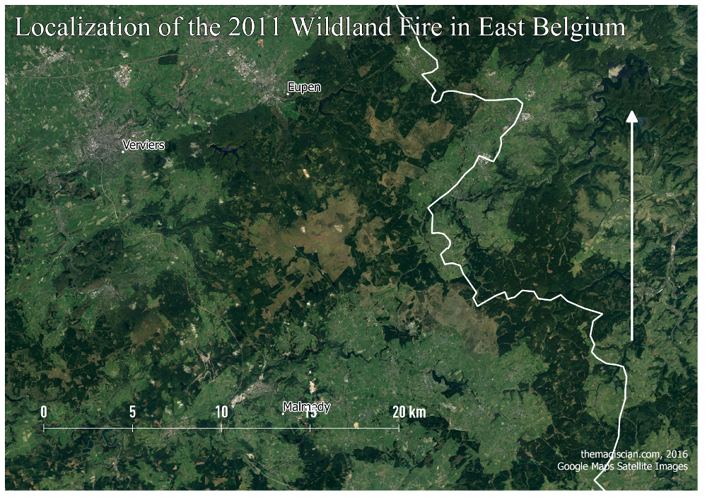
Our study area in the High Fens.
And here a look on the field.
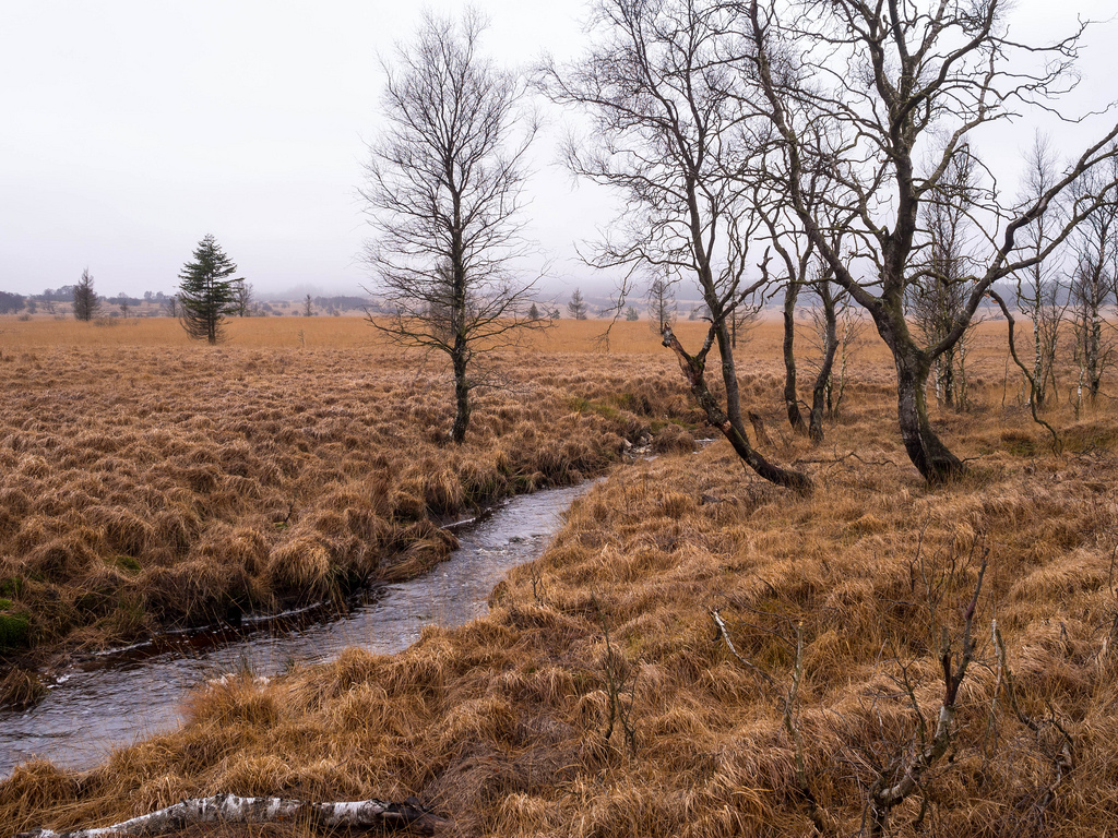
As you can see, in Belgian’s high altitudes (over 600m (2000 ft) above sea level), the landscape is a type of grassy wetland with sparsely densed trees. That’s why we’re talking about wildland fire instead of “forest fire” in this article.
Our first step is to get a sample data of the region taken BEFORE the wildland fire and to compare it with data AFTER.
Getting the data
Landsat 7 Data are freely available on the USGS Website: http://landsatlook.usgs.gov/viewer.html. Just create an account and you’re ready to go!
Do pan to our area of interest and specify the search criteria as following:
- For the first image (“before”): Date: between 01/04/2011 and 24/04/2011.
- And for the second image (“after”): Date: between 01/05/2011 and 31/05/2011.
Proceed to check out and choose the full L1 data.
In our case we got Landsat 7 imageries from timestamp 2011-04-19 10:21:39.5662647Z and the timestamp for the second one is 2011-05-05 10:21:40.9679034Z. An image just 6 days before the fire and the second 9 days after.
Here’s what the unzipped data look like. Each band is in a separate file. For details about the spectral scope of each band, please refer to this page.

Data loading
We decide to store the acquired data into a PostGIS database. In fact, we do not necessarily need a database for storing and processing just two images. We want just to show PostGIS capabilities for Remote Sensing processing.
Create the database (here wildlandfire) and enable the raster capabilities with following query.
psql -f /usr/share/postgresql/9.4/contrib/postgis-2.1/rtpostgis.sql -Upostgres -h<ip-address> -dwildlandfire
We use the utility raster2pgsql and here’s our commands:
raster2pgsql -c -C -s 32631 -f rast -F -I -M -t 100x100 /path_to_data/0008_LANDSAT7_ANALYSIS/April/LE71970252011109ASN00_B1.TIF
public.april_b1 | psql -Uthemagiscian -hip-address -dwildlandfire
 /path_to_data ip-address
raster2pgsql -d -C -s 32631 -f rast -F -I -M -t 100x100 /path_to_data/0008_LANDSAT7_ANALYSIS/April/LE71970252011109ASN00_B2.TIF
public.april_b2 | psql -Uthemagiscian -hip-address -dwildlandfire
 /path_to_data ip-address
raster2pgsql -d -C -s 32631 -f rast -F -I -M -t 100x100 /path_to_data/0008_LANDSAT7_ANALYSIS/April/LE71970252011109ASN00_B3.TIF
public.april_b3 | psql -Uthemagiscian -hip-address -dwildlandfire
[...]
Notice in bold the naming convention we adopted for the tables in the database: month + b (for band) + band number.
Here is the help guide for this command to know what parameters I used. The interesting parameters here is the -t 100×100. We create 100×100 pixels tiles on the whole image. In other words, every row in the different tables corresponds to one tile.
We noticed during our later analyses that the tiles for every raster image were not surimposed, which makes the calculations difficult. We need to make sure they are! Here’s the alignment problem.

To overcome this issue, we create a union of all the layers we need.
DROP TABLE may_b4_union;
CREATE TABLE may_b4_union AS
SELECT 1 as rid, ST_Union(rast,1) rast
FROM may_b4;
ALTER TABLE may_b4_union ADD CONSTRAINT may_b4_union_pk PRIMARY KEY (rid);

DROP TABLE april_b4_union;
CREATE TABLE april_b4_union AS
SELECT 1 as rid, ST_Union(rast,1) rast
FROM april_b4;
ALTER TABLE april_b4_union ADD CONSTRAINT april_b4_union_pk PRIMARY KEY (rid);

DROP TABLE april_b7_union;
CREATE TABLE april_b7_union AS
SELECT 1 as rid, ST_Union(rast,1) rast
FROM april_b7;
ALTER TABLE april_b7_union ADD CONSTRAINT april_b7_union_pk PRIMARY KEY (rid);

DROP TABLE may_b7_union;
CREATE TABLE may_b7_union AS
SELECT 1 as rid, ST_Union(rast,1) rast
FROM may_b7;
ALTER TABLE may_b7_union ADD CONSTRAINT may_b7_union_pk PRIMARY KEY (rid);
Remote Sensing Analyses
Our goal is to identify the area of the burnt land. As we’re using Landsat 7 images, we know from the metadata that the images are already georeferenced and were calibrated. This is a big advantage as we do not need to go through all of this for this tutorial.
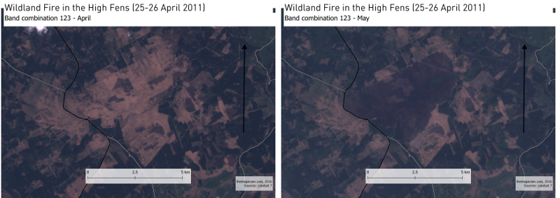
True Color
See how our area look from the sky in true color, that means, band combination 123. We used QGIS for all the visualisations.
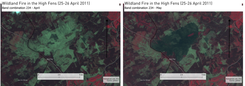
False Color
The false color 234 band combination gives us also a sign that something happened here. Notice also how the vegetation grows during these 15 days during the Spring (especially visible in the North West).
Band combination 247: Soil and vegetation moisture
This is maybe the best band combination for studying soil moisture. It involves swir band n°7.
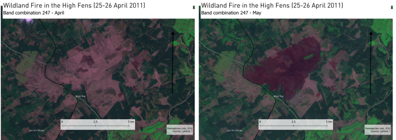
Healthy vegetation is bright green and the overall surroundings become greener as Spring continues. The vegetation at the bord of the burnt area is darker because is heavily planted with Picea abies. The pink areas are barren soils and fires appear red. The burnt area is clearly highlighted.
Band combination 357: Forest Fires
A last band combination presented here is the 357 especially suited for forest fires. It involves
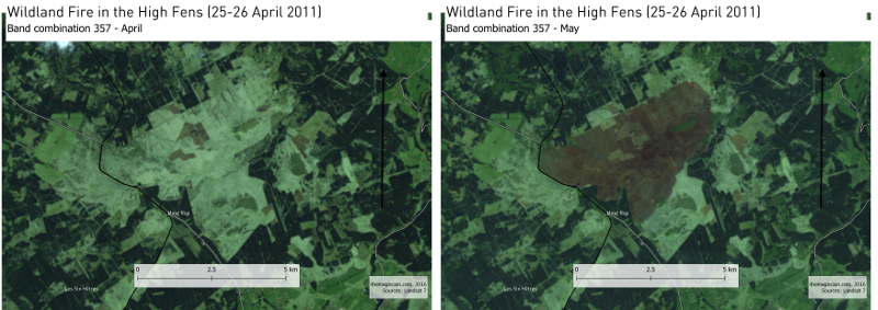
This band combination has the particularity to represent hot surfaces in shades of red of yellow, as is hence well suited for monitoring forest fires. In our case, the wildland fire is over but we can still notice a hotter surface temperature in our area.
Identify The Fire Extent
For identifying the wildland fire extent, we know from Remote Sensing lectures that we have several indexes we could use, like the Normalized Burn Ratio (NBR).
NBR = (NIR - SWIR) / (NIR + SWIR)
Note that indexes could have been used like the Burn Area Index (BAI), Normalized Burn Ratio Thermal 1 (NBRT1), etc.
We apply this calculation for both the BEFORE and the AFTER images.
For Landsat 7, the NIR band is the fourth one and the SWIR is the band n°7. As we know from our naming patterns, and according to the formula, our SQL request looks like this.
DROP TABLE april_fire_nbr;
CREATE TABLE april_fire_nbr AS
SELECT 1 rid, ST_MapAlgebra(arast, 1, brast, 1, '([rast1] - [rast2]) / ([rast1] + [rast2])', '32BF') AS rast
FROM (SELECT a.rid, a.rast as arast, b.rast as brast FROM april_b4_union a INNER JOIN april_b7_union b ON a.rid = b.rid) AS joined;
ALTER TABLE april_fire_nbr ADD CONSTRAINT april_fire_nbr_pk PRIMARY KEY (rid);

DROP TABLE may_fire_nbr;
CREATE TABLE may_fire_nbr AS
SELECT 1 rid, ST_MapAlgebra(arast, 1, brast, 1, '([rast1] - [rast2]) / ([rast1] + [rast2])', '32BF') AS rast
FROM (SELECT a.rid, a.rast as arast, b.rast as brast FROM may_b4_union a INNER JOIN may_b7_union b ON a.rid = b.rid) AS joined;
ALTER TABLE may_fire_nbr ADD CONSTRAINT may_fire_nbr_pk PRIMARY KEY (rid);
Here are the colorized results.
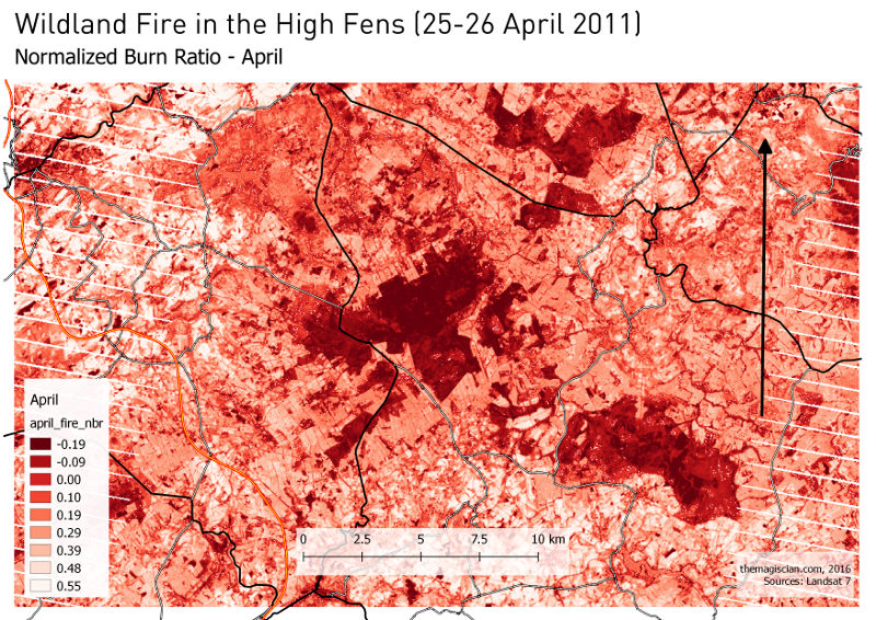
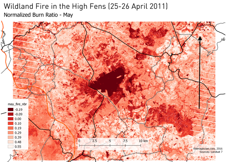
We then do an addition with these two results. As we can see, in both images the burn area pixels are in the most negative values (obvisouly this shouldn’t be the case – but, remember, we are in the case of a wildland fire and not forest fire).
DELTA_NBR = APRIL_NBR + MAY_NBR

DROP TABLE delta_fire_nbr;
CREATE TABLE delta_fire_nbr AS
SELECT 1 rid, ST_MapAlgebra(arast, 1, brast, 1, '([rast1] + [rast2])', '32BF') AS rast
FROM (SELECT a.rid, a.rast as arast, b.rast as brast FROM april_fire_nbr a INNER JOIN may_fire_nbr b ON a.rid = b.rid) AS joined;
ALTER TABLE delta_fire_nbr ADD CONSTRAINT delta_fire_nbr_pk PRIMARY KEY (rid);
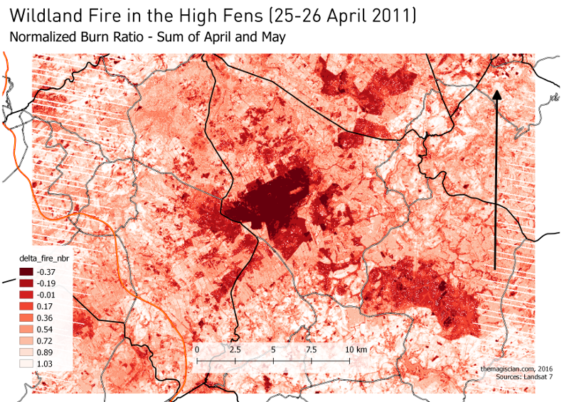
The burnt area is much more clear now. To determine from which pixel value we can assume there’s a burnt land is done via a try and error. We found out that pixel values less than -.35 is a good catch.
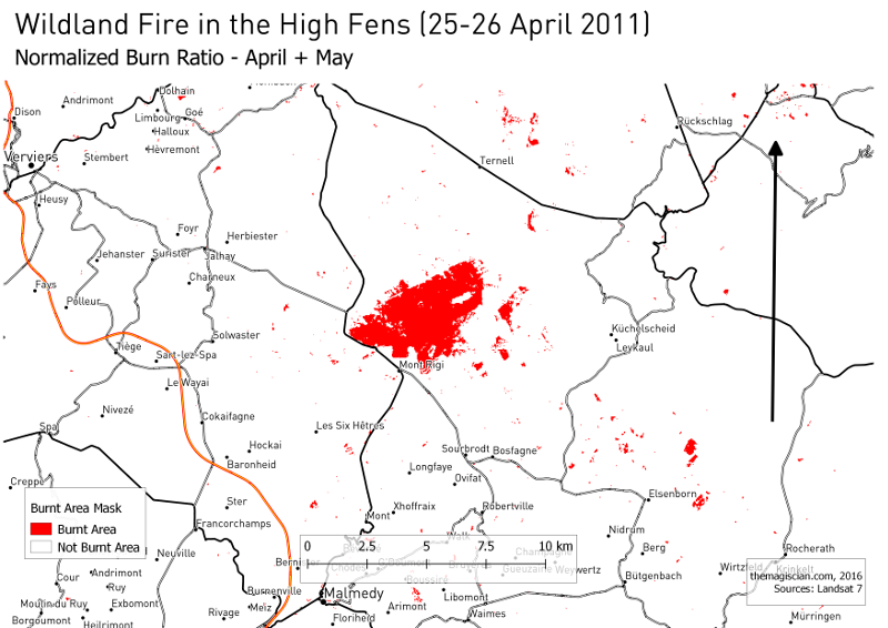
From there, we “just” need to count the pixels that are in red (< -.35). In our sql query, we do restraint the calculations to the burnt area. We know for sure that the burnt area lies between the polygon defined by the coordinates.
-- Count the burned pixels only in the fire_area
WITH fire_area AS (SELECT 1 rid,
ST_Clip(rast, ST_GeomFromText('POLYGON((715633.942 5599374.235, 715633.942 5604869.328, 722213.940 5604869.328,
722152.198 5599374.235, 715633.942 5599374.235))', 32631)) rast FROM delta_fire_nbr)

SELECT sum(total)*900/10000 || ' ha' FROM
(SELECT (pvc).VALUE, (pvc).COUNT total
FROM (SELECT ST_ValueCount(rast) As pvc FROM fire_area) As a
WHERE (pvc).VALUE < -.35
ORDER BY (pvc).value) As b;
We find out 1316 ha, which is the result given by the firefighter in the newspapers. For the calculation, we multiply the number of pixels by 900m² (30 being the resolution of Landsat 7 imageries). We divide it the by 10 000 to have the unit in hectares.
Notice that the result could have more precise if we had performed pan-sharpening operations on all the input data.
Conclusion
With the available Landsat 7 data, the GIS tools such as PostGIS and QGIS, and Remote Sensing techniques, we were able to isolated the wildland fire burnt area and to calculate its extent.
Bonus
Just a month after the fire, Mother Nature took back her Rights.

Thanks a lot!
Cheers,
Daniel
Leave a Reply