Everyone who went cycling in Belgium knows that the famous quote from Jacques Brel “Le plat pays qui est le mien” is far from being true! Belgium is globally a flat land with the highest point sitting at 694m above sea level, this is true, but once on a bike you notice immediately that painfull slopes are just around the corners. Taking into account the elevation and the slopes is important in routing algorithms.
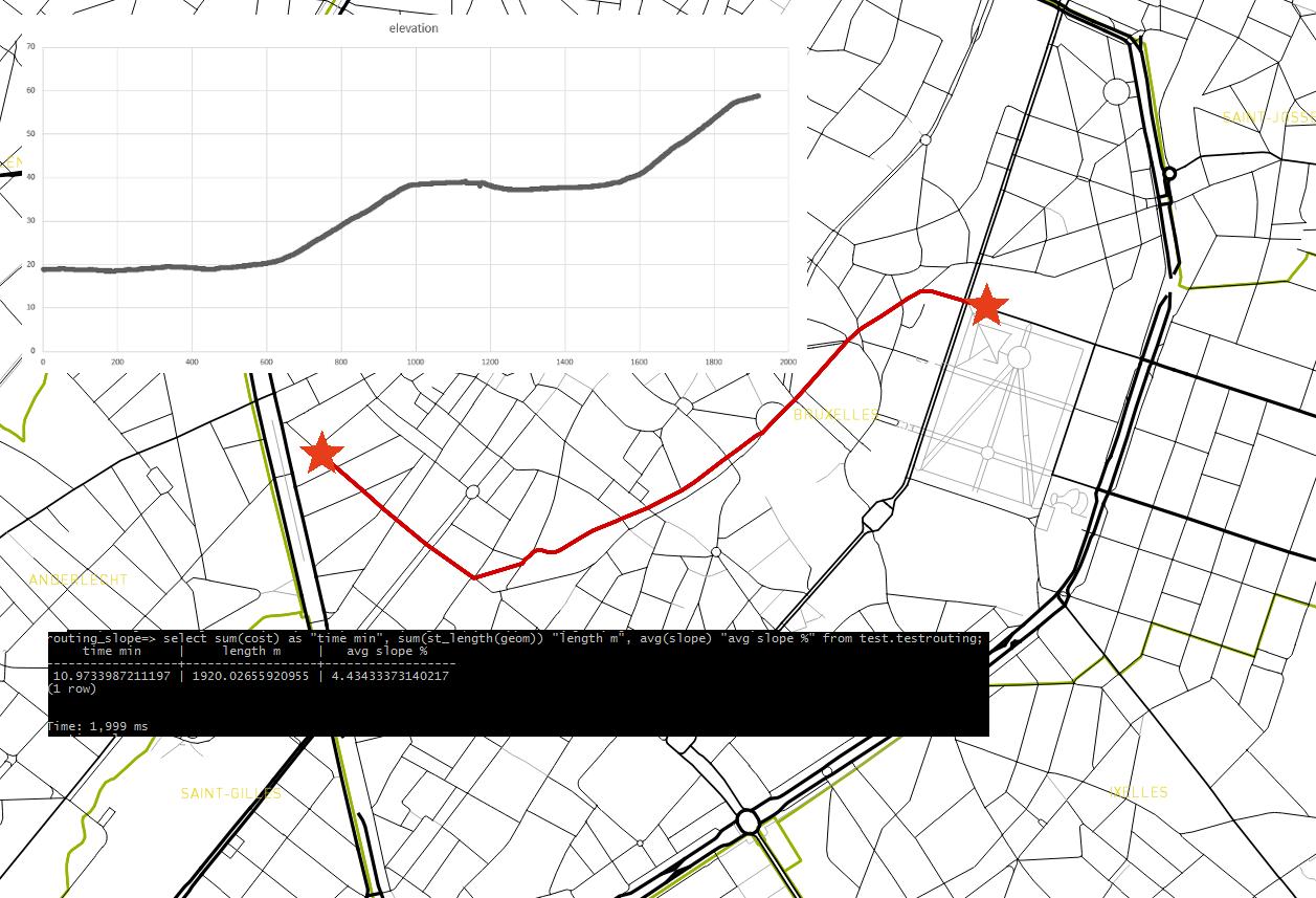
In this article, we will analyze the shortest cycling routes in Brussels by taking into account the slopes. Elderly people who wants to visit our Belgian Capital City by bike would be interested in such a map to choose going from A to B by the route offering the smallest slopes. In the following screenshot, we follow a bike going from the Bodeghem quarter to Rue de la Loi where the highest Belgian Institutions are located. The journey takes about 10 min by bike and is 1920 meters long. In the longitudinal profile, we see where the slopes are located and the elevation goes from 20m at the start to 60m at the arrival.
Routing with slope
For our exercice, with need two set of data: A DEM covering Brussels and the road network. Notice that the tools we use are PostGIS and QGIS for visualizing the results.
DATA
The DEM of 1 m resolution is coming from the agiv.be website. A real treasure having a DEM of 1m resolution in XY and 1mm in Z! Our network data comes from OpenStreetMap.
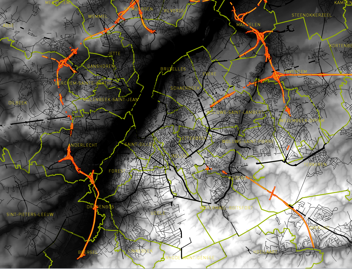
DEM and OSM
Database preparation
As always in our articles, we detail the steps to setup the environment.
Connect to PostgreSQL and create the database.
psql -Upostgres -h<ip>
CREATE DATABASE routing_slope WITH OWNER themagiscian;
Connect to the database in order to activate the extensions
\c routing_slope
CREATE EXTENSION postgis;
CREATE EXTENSION hstore;
CREATE EXTENSION pgrouting;
Connect then to the database with your user
\c routing_slope themagiscian
Data import
Our database is up and ready. Let’s import our data!
The DEM is imported using the raster2pgsql tool.
raster2pgsql -c -C -s 31370 -f rast -F -I -M -t 100x100 DHMVIIDTMRAS1m_k31.tif public.brussels_dem
| psql -Uthemagiscian -h<ip> -drouting_slope
If you did not already download the OSM data from Brussels, here is the snippet to do so, provided you have wget installed.
wget --progress=dot:mega -O "brussels2.osm"
"http://www.overpass-api.de/api/xapi?*[bbox=4.20914,50.766,4.5401,50.93593][@meta]"
From there, import the dataset into the database.
osm2pgsql -d routing_slope -H <ip> -U themagiscian -P 5432 -W -S default.style --hstore brussels.osm
Database cleaning
Our imports created a lot of stuff in our database. Here we’re cleaning things up.
osm2pgsql assigns names to the tables. We make them more user friendly.
ALTER TABLE planet_osm_line RENAME TO streets;
All the tables we do not need are thrown away.
DROP TABLE planet_osm_nodes;
DROP TABLE planet_osm_point;
DROP TABLE planet_osm_polygon;
DROP TABLE planet_osm_rels;
DROP TABLE planet_osm_roads;
DROP TABLE planet_osm_ways;
We used to name the geomety column ‘geom’
ALTER TABLE streets RENAME way TO geom;
As OSM comes with a tremendous amount of columns we do not need, we decide also to throw away all the fields we do not need.
ALTER TABLE streets DROP COLUMN access, DROP COLUMN "addr:housename", DROP COLUMN "addr:housenumber",
DROP COLUMN "addr:interpolation", DROP COLUMN admin_level, DROP COLUMN aerialway, DROP COLUMN aeroway,
DROP COLUMN amenity, DROP COLUMN area, DROP COLUMN barrier, DROP COLUMN brand, DROP COLUMN boundary,
DROP COLUMN building, DROP COLUMN construction, DROP COLUMN covered, DROP COLUMN culvert, DROP COLUMN cutting,
DROP COLUMN denomination, DROP COLUMN disused, DROP COLUMN embankment, DROP COLUMN foot,
DROP COLUMN "generator:source", DROP COLUMN harbour, DROP COLUMN historic, DROP COLUMN horse,
DROP COLUMN intermittent, DROP COLUMN junction, DROP COLUMN landuse, DROP COLUMN layer, DROP COLUMN leisure,
DROP COLUMN lock, DROP COLUMN man_made, DROP COLUMN military, DROP COLUMN motorcar, DROP COLUMN name,
DROP COLUMN "natural", DROP COLUMN office, DROP COLUMN operator, DROP COLUMN place, DROP COLUMN population,
DROP COLUMN power, DROP COLUMN power_source, DROP COLUMN public_transport, DROP COLUMN railway, DROP COLUMN ref,
DROP COLUMN religion, DROP COLUMN route, DROP COLUMN service, DROP COLUMN shop, DROP COLUMN sport,
DROP COLUMN surface, DROP COLUMN toll, DROP COLUMN tourism, DROP COLUMN "tower:type", DROP COLUMN tracktype,
DROP COLUMN water, DROP COLUMN waterway, DROP COLUMN wetland, DROP COLUMN width, DROP COLUMN wood,
DROP COLUMN z_order, DROP COLUMN way_area;
That’s all for the cleaning.
Combine Slope and Elevation Data with the Streets
That’s a tough part: Our DEM contains the elevation data and our streets are the basis of the network. Furthermore, we need to extract the slopes from the DEM and assign these values to the street segments. A lot of processing work for the computer and it is therefore important to optimize the requests in order to make processing times quicker.
First things first, we create a staging schema where we will stuff all our data and intermediary data.
CREATE SCHEMA staging;
The first step is to create a dem table of the area. In other words, we only consider pixel data on the Brussels Region
CREATE TABLE staging.brussels_dem_intersect AS
SELECT DISTINCT b.rid, b.rast rast
FROM brussels_dem b, pentagon p
WHERE ST_Intersects(b.rast, ST_Transform(p.geom,31370));
The Slopes are extracted from the DEM using the ST_Slope function.
CREATE TABLE staging.brussels_slope AS SELECT ST_Slope(b.rast, 1, '32BF', 'PERCENT', 1.0) rast FROM brussels_dem b;
ALTER TABLE staging.brussels_slope ADD COLUMN rid SERIAL PRIMARY KEY;
CREATE INDEX staging_brussels_slope_gix ON staging.brussels_slope USING GIST(st_convexhull(rast));
The ST_Slope takes as argument the raster field, the band number, the data encoding and the vertical exaggeration. The output data has to be indexed.
Our next tactic is to vectorize the Slope dataset. In other words, the pixels becomes squares and keep their slope values. You see it coming, we will in a later step extract these slope information with an intersection with the street layer.
Here’s the vectorization of the Slope dataset.
CREATE TABLE staging.brussels_slope_vector_square AS SELECT (ST_DumpAsPolygons(bslope.rast)).val slope,
(ST_DumpAsPolygons(bslope.rast)).geom geom FROM staging.brussels_slope bslope;
ALTER TABLE staging.brussels_slope_vector_square ADD COLUMN id SERIAL PRIMARY KEY;
CREATE INDEX staging_brussels_slope_vector_square_gix ON staging.brussels_slope_vector_square USING GIST(geom);
We do exactly the same with our original DEM.
CREATE TABLE staging.brussels_dem_vector_square AS SELECT (ST_DumpAsPolygons(b.rast)).val elevation,
(ST_DumpAsPolygons(b.rast)).geom geom FROM staging.brussels_dem_intersect b;
ALTER TABLE staging.brussels_dem_vector_square ADD COLUMN id SERIAL PRIMARY KEY;
CREATE INDEX brussels_dem_vector_square_gix ON staging.brussels_dem_vector_square USING GIST(geom);
Now we can intersect the vector layers and grab the Slope information to put them into the Streets layer. Notice that we cut each Streets line at the intersection. As the resolution of our Slope dataset is 1m in XY, our line will be cut in the order. Each small piece of street will have a different Slope value. A BIG AMOUNT OF STREETS PARTS WE’RE CREATING!
CREATE TABLE staging.streets_slope AS SELECT s.osm_id, bslopev.slope, belevv.elevation,
ST_Intersection(ST_Transform(s.geom, 31370), bslopev.geom) AS geom FROM streets s,
staging.brussels_slope_vector_square bslopev, staging.brussels_dem_vector_square belevv
WHERE ST_Intersects(ST_Transform(s.geom, 31370), bslopev.geom)
AND ST_Intersects(ST_Transform(s.geom, 31370), belevv.geom);
ALTER TABLE staging.streets_slope ADD COLUMN id SERIAL PRIMARY KEY;
CREATE INDEX staging_streets_slope_gix ON staging.brussels_slope_vector_square USING GIST(geom);
Notice that we make several times use of the ST_Transform function. This is mandatory because our datasets are in different SRS. Our DEM is in 31370 (Belgian Lambert 72) and the Streets from OpenStreetMap are in 3857. For the intersection function to work, both have to be in the same SRS. For you information, this takes the longest processing time. Be patient.
Our next steps is to add the Elevation information to the already cut in small pieces Streets layer.
ALTER TABLE staging.streets_slope ADD COLUMN elevation double precision;
UPDATE staging.streets_slope ss SET elevation = bdem.elevation FROM staging.brussels_dem_vector_square bdem
WHERE ST_Intersects(ST_Transform(ss.geom, 31370), bdem.geom);
UPDATE stagingt.streets_slope ss SET elevation = bdem.elevation FROM stagingt.brussels_dem_vector_square bdem
WHERE (ss.id = 92084) AND ST_Intersects(ST_Transform(ss.geom, 31370), bdem.geom);
We do add the information by adding a new field and filling it with data coming from our vectorized DEM.
Create Network
Our Streets layer is ready to be used!
We need, first, to add new columns to our Streets layer. These columns will receive the ids of both boundary points. The source and target point of the line.
ALTER TABLE staging.streets_slope ADD COLUMN "source" integer;
ALTER TABLE staging.streets_slope ADD COLUMN "target" integer;
CREATE INDEX staging_streets_slope_idx ON staging.streets_slope(id);
From there, we create the topology using the pgr_createTopology function.
SELECT pgr_createTopology('staging.streets_slope', 0.0000001, 'geom', 'id');
CREATE INDEX staging_streets_slope_source_idx ON staging.streets_slope("source");
CREATE INDEX staging_streets_slope_target_idx ON staging.streets_slope("target");
The cost of our streets, that mean, the constraint used to calculate the shortest routes, is decided to be the time, in minutes, it takes to cross it.
ALTER TABLE staging.streets_slope ADD COLUMN time_min double precision;
We arbitrary decide that a bike rides at 15km/h when it is flat. This speed goes linearily down to 5 km/h at a slope of 10%. Here are the formulae to fill these fields.
UPDATE staging.streets_slope SET time_min = (ST_Length(geom) / ((-1 * slope + 15) * 1000 / 60)) WHERE slope <= 10;
UPDATE staging.streets_slope SET time_min = (ST_Length(geom) / (5 * 1000 / 60)) WHERE slope > 10;
ALTER TABLE staging.streets_slope ADD COLUMN reverse_time_min double precision;
UPDATE staging.streets_slope SET reverse_time_min = time_min;
ALTER TABLE streets_slope_vertices_pgr SET SCHEMA staging;
ALTER TABLE staging.streets_slope_vertices_pgr RENAME the_geom TO geom;
Notice how we do aesthetics by putting the streets_slope_vertices back to the staging schema and the by default naming ‘the_geom’ becomes ‘geom’.
As we already did it in a previous article about the routing in Brisbane, we defined a wrapper function that makes it possible to calculate the least costing route from A to B. This wrapper function takes as input the x and y from the start and arrival points. From there, it chooses the corresponding nodes in the built network and calculates the lest costing route using the famous and the never out of fashion Dijkstra algorithm.
CREATE OR REPLACE FUNCTION pgr_fromAtoB(
 IN tbl varchar,
 IN x1 double precision,
 IN y1 double precision,
 IN x2 double precision,
 IN y2 double precision,
 OUT seq integer,
 OUT id integer,
 OUT name text,
 OUT heading double precision,
 OUT cost double precision,
 OUT geom geometry
 )
 RETURNS SETOF record AS
 $BODY$
 DECLARE
 sql text;
 rec record;
 source integer;
 target integer;
 point integer;

BEGIN
 -- Find nearest node
 EXECUTE 'SELECT id::integer FROM staging.streets_slope_vertices_pgr
 ORDER BY geom <-> ST_Transform(ST_GeometryFromText(''POINT('
 || x1 || ' ' || y1 || ')'',4326), 31370) LIMIT 1' INTO rec;
 source := rec.id;

EXECUTE 'SELECT id::integer FROM staging.streets_slope_vertices_pgr
 ORDER BY geom <-> ST_Transform(ST_GeometryFromText(''POINT('
 || x2 || ' ' || y2 || ')'',4326), 31370) LIMIT 1' INTO rec;
 target := rec.id;

-- Shorstaging path query (TODO: limit extent by BBOX)
 seq := 0;
 sql := 'SELECT id, geom, osm_id::text AS name, cost, reverse_time_min, source, target,
 ST_Reverse(geom) AS flip_geom FROM ' ||
 'pgr_dijkstra(''SELECT id, source::int, target::int, '
 || 'time_min::float AS cost, reverse_time_min::float AS reverse_cost FROM '
 || (tbl) || ''', '
 || source || ', ' || target
 || ' , false, true), '
 || (tbl) || ' WHERE id2 = id ORDER BY seq';

-- Remember start point
 point := source;

FOR rec IN EXECUTE sql
 LOOP
 -- Flip geometry (if required)
 IF ( point != rec.source ) THEN
 rec.geom := rec.flip_geom;
 point := rec.source;
 ELSE
 point := rec.target;
 END IF;

-- Calculate heading (simplified)
 EXECUTE 'SELECT degrees( ST_Azimuth(
 ST_StartPoint(''' || rec.geom::text || '''),
 ST_EndPoint(''' || rec.geom::text || ''') ) )'
 INTO heading;

-- Return record
 seq := seq + 1;
 id := rec.id;
 name := rec.name;
 cost := rec.cost;
 geom := rec.geom;
 RETURN NEXT;
 END LOOP;
 RETURN;
 END;
 $BODY$
 LANGUAGE 'plpgsql' VOLATILE STRICT;
The cost we defined is the time_min, the time it takes to cross each Streets segment in minutes.
Test the Routing environment!
The last and funniest part is testing out our infrastructure! From QGIS, we gather the long/lat coordinate from our points of interesting and stuff it into our wrapper function!
DROP TABLE staging.stagingrouting;
CREATE TABLE staging.stagingrouting AS SELECT p.seq, p.id, p.name, p.heading, p.cost, s.slope, s.elevation, p.geom
FROM pgr_fromAtoB('staging.streets_slope',4.34260,50.84224,4.35268,50.85145) p JOIN staging.streets_slope s ON p.id=s.id;
The following query gives us more details about the route the algorithm chose.
select sum(cost) as "time min", sum(st_length(geom)) "length m", avg(slope) "avg slope %" from test.testrouting;

 time min | length m | avg slope %
------------------+------------------+------------------
 10.9733987211197 | 1920.02655920955 | 4.43433373140217
(1 row)
Important to notice: the average slope is not quite correct. To have the average slope, we need to ponderate each Streets segment with its length. Here it is only an arithmetic average, which is not correct.
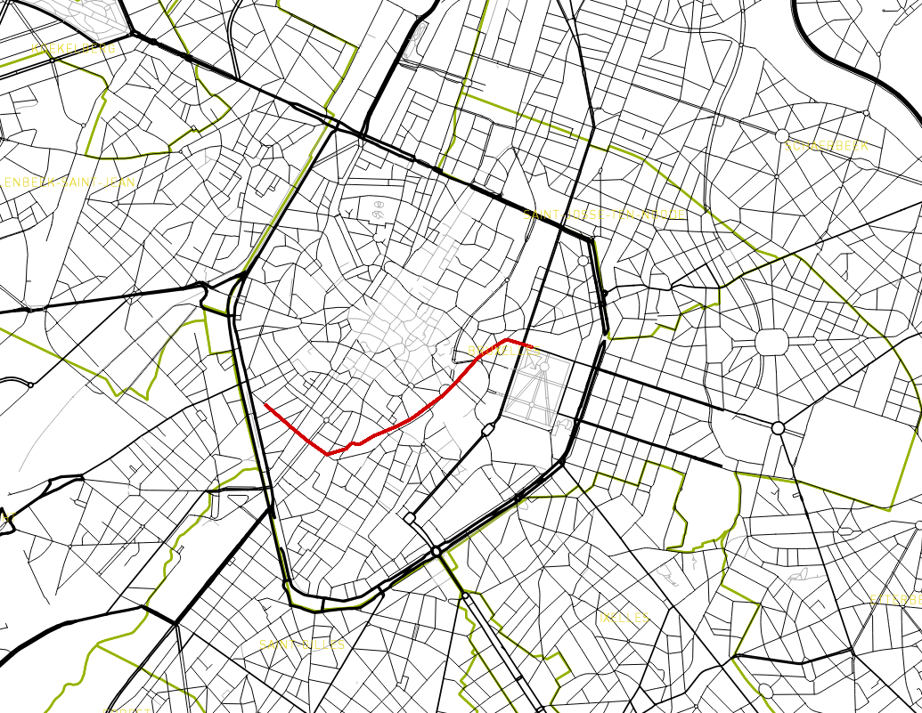
Routing
Get the Longitudinale Profile
An important piece of our developments is to create the longitudinal profile. Here, Excel comes into play with its charting capabilities.
Data are extracted to a CSV file using ogr2ogr.
ogr2ogr -progress -sql "select seq, cost, heading, st_length(geom) length, elevation, slope from test.testrouting"
-f CSV routing.csv PG:"host='<ip>' dbname=routing_slope user='themagiscian' password='*****'"
From there, we plot the data on a graph and we obtain the following one.
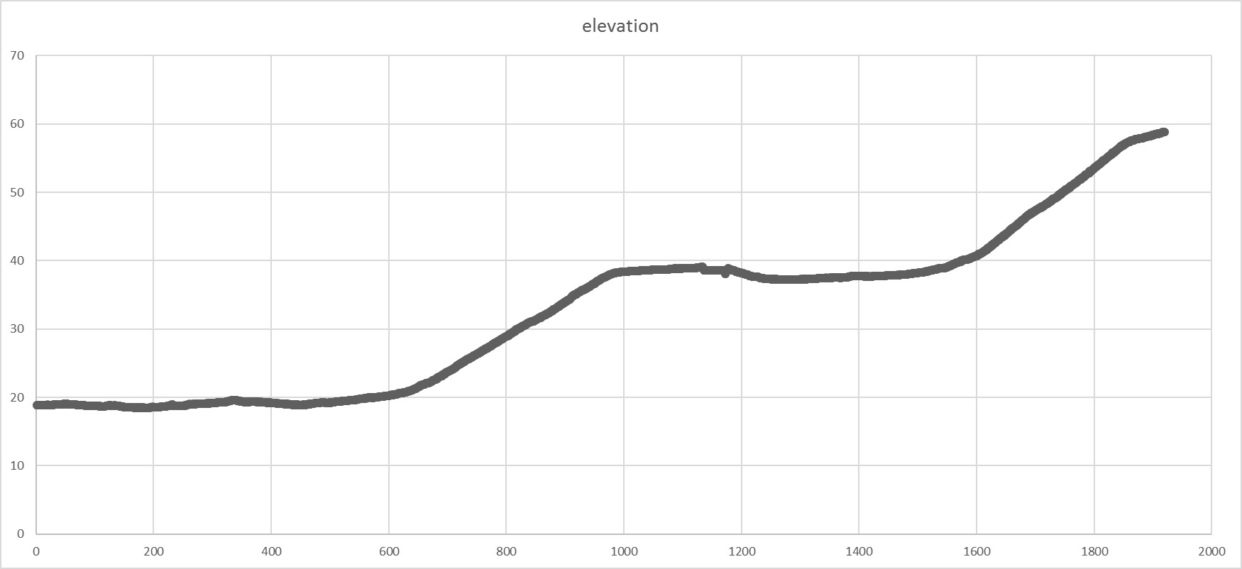
Longitudinal Profile
Conclusions
With free data (AGIV, OSM) and free tools (PostGIS, QGIS, ogr2ogr), we were able to create a routing infrastructure that takes into account the slope in the Best route alternative algorithm. Possible applications could be for elderly people who visit Brussels by bike for them to take the least effort-demand route.
Cheers,
Daniel, themagiscian.com
Leave a Reply